<?xml version="1.0" encoding="utf-8"?><feed xmlns="http://www.w3.org/2005/Atom" ><generator uri="https://jekyllrb.com/" version="3.10.0">Jekyll</generator><link href="https://thomasgraceman.github.io/feed.xml" rel="self" type="application/atom+xml" /><link href="https://thomasgraceman.github.io/" rel="alternate" type="text/html" /><updated>2026-09-14T21:06:47+00:00</updated><id>https://thomasgraceman.github.io/feed.xml</id><title type="html">A steeper descent</title><subtitle>Research blog on theoretical computer science — metric embeddings, sparsification, generic chaining, and approximation algorithms. Notes on papers and books by Taha Hoseinpour.</subtitle><author><name>Taha</name><email>tahahoseinpourasli@gmail.com</email></author><entry><title type="html">And god said let there be dijkstra</title><link href="https://thomasgraceman.github.io/posts/and-god-said-let-there-be-dijkstra/" rel="alternate" type="text/html" title="And god said let there be dijkstra" /><published>2026-08-22T00:00:00+00:00</published><updated>2026-08-22T00:00:00+00:00</updated><id>https://thomasgraceman.github.io/posts/And-god-said-let-there-be-dijkstra</id><content type="html" xml:base="https://thomasgraceman.github.io/posts/and-god-said-let-there-be-dijkstra/"><![CDATA[<p>Alright, in this work I want to explain the seminal work of Jittat Fakcharoenphol and Satish Rao in 2006, devising the algorithm of FR-Dijkstra, which is so insightful and meaningful.</p>

<p>A disclaimer: I still don’t have full command over the concepts of the papers, and this post may be subject to a future update, so feel free to mention if I got something wrong.</p>

<p>So, what if we have a very dense graph maybe and we want to beat the Dijkstra algorithm, then how can we do it? At least in the planar case. The answer is to sparsify the initial object a bit, and instead decompose the graph into local pieces in which you have a rough information of, you use that to traverse the global structure in a way, and when needed you use that to compute the true shortest path, by the local graph where using Dijkstra or Bellman–Ford is efficient.</p>

<p>So in this post I am going to assume the existence of \(r\)-separators.</p>

<p>Ok, let’s review the definition of \(r\)-separators:</p>

<p>Let \(\Sigma\) be a simple planar map with weighted darts; for now we’ll assume that all edge weights are non-negative. If necessary, add infinite-weight edges so that \(\Sigma\) is a simple triangulation.</p>

<p>Recall that a good \(r\)-division of \(\Sigma\) is a subdivision of \(\Sigma\) into \(O(n/r)\) pieces \(R_1, R_2, \ldots\) satisfying three conditions:</p>

<ul>
  <li>Each piece has \(O(r)\) vertices.</li>
  <li>Each piece has \(O(\sqrt{r})\) boundary vertices (that is, vertices that are shared with other pieces).</li>
  <li>Each piece has \(O(1)\) holes (faces of the piece that are not faces of \(\Sigma\)).</li>
</ul>

<p><strong>Recall.</strong>
An MSSP (Multiple-Source Shortest Paths) data structure for a planar graph with \(n\) vertices can be constructed in \(O(n\log n)\) preprocessing time and space, and supports distance queries in \(O(\log n)\) time. The queries are restricted to sources lying on a single face.</p>

<p>For a piece \(R_i\) of an \(r\)-division, we have \(O(r)\) vertices and \(O(\sqrt{r})\) boundary vertices. Since the boundary vertices lie on the constant number of holes of the piece, we can construct an MSSP data structure for \(R_i\) and use it to compute all boundary-to-boundary distances.</p>

<p>The preprocessing time for one piece is</p>

\[O(r\log r).\]

<p>There are \(O(\sqrt{r})\) boundary vertices, so there are</p>

\[O(\sqrt{r})^2 = O(r)\]

<p>boundary-to-boundary distance queries. Each query takes \(O(\log r)\) time, giving another</p>

\[O(r\log r)\]

<p>time per piece. Hence, the total time for one piece is</p>

\[O(r\log r).\]

<p>Since the \(r\)-division contains \(O(n/r)\) pieces, the total time to construct the dense distance graph is</p>

\[O\left(\frac{n}{r}\cdot r\log r\right) = O(n\log r).\]

<p><strong>Dense Distance Graph.</strong>
For each piece \(R_i\), we construct a weighted clique on its boundary vertices. For every pair of boundary vertices \(u,v\in\partial R_i\), the corresponding dart has weight</p>

\[w_i(u,v)=d_{R_i}(u,v),\]

<p>where \(d_{R_i}(u,v)\) denotes the shortest-path distance from \(u\) to \(v\) using only vertices and edges of \(R_i\).</p>

<p>The dense distance graph is the union of these \(O(n/r)\) weighted cliques.</p>

<p>Each piece has \(O(\sqrt{r})\) boundary vertices, so the total number of distinct boundary vertices is</p>

\[n' = O\left(\frac{n}{r}\cdot\sqrt{r}\right) = O\left(\frac{n}{\sqrt{r}}\right).\]

<p>Furthermore, each piece contributes</p>

\[O((\sqrt{r})^2)=O(r)\]

<p>weighted darts. Therefore, over all \(O(n/r)\) pieces,</p>

\[m' = O\left(\frac{n}{r}\cdot r\right) = O(n).\]

<p>Thus the dense distance graph has</p>

\[n'=O\left(\frac{n}{\sqrt{r}}\right) \qquad\text{and}\qquad m'=O(n)\]

<p>and can be constructed in</p>

\[O(n\log r)\]

<p>time.</p>

<p>So, how can we use this rough structure to beat Dijkstra in an efficient manner? Let’s do what one naturally may do:</p>

<p><strong>Theorem.</strong>
Given any planar map \(\Sigma\) with non-negative lengths on its edges, we can compute the shortest paths from any vertex \(s\) to every other vertex of \(\Sigma\) in \(O(n\log\log n)\) time.</p>

<p><strong>Proof.</strong>
We begin by triangulating \(\Sigma\) in \(O(n)\) time, building a good \(r\)-division for the resulting triangulation in \(O(n)\) time, and building the dense distance graph for the \(r\)-division in \(O(n\log r)\) time, for some parameter \(r\) to be determined. In the top-level recursive call to build the good \(r\)-division, we artificially declare \(s\) to be a boundary vertex, so that it survives as a vertex in the dense-distance graph.</p>

<p>Next, we compute the shortest-path distance from \(s\) to every boundary vertex of the \(r\)-division by running Dijkstra’s algorithm on the dense distance graph. If we implement Dijkstra’s algorithm using Fibonacci heaps, this step takes</p>

\[O(n'\log n' + m') = O\left(\frac{n}{\sqrt{r}}\log n+n\right)\]

<p>time, since</p>

\[n'=O\left(\frac{n}{\sqrt{r}}\right) \qquad\text{and}\qquad m'=O(n).\]
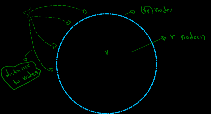
<p><img src="/images/fr-r-division.png" alt="An r-division piece: about r interior nodes, O(sqrt r) boundary nodes, and distances from a source s into the boundary" style="max-width: 520px; height: auto; display: block; margin: 1.5em auto;" /></p>

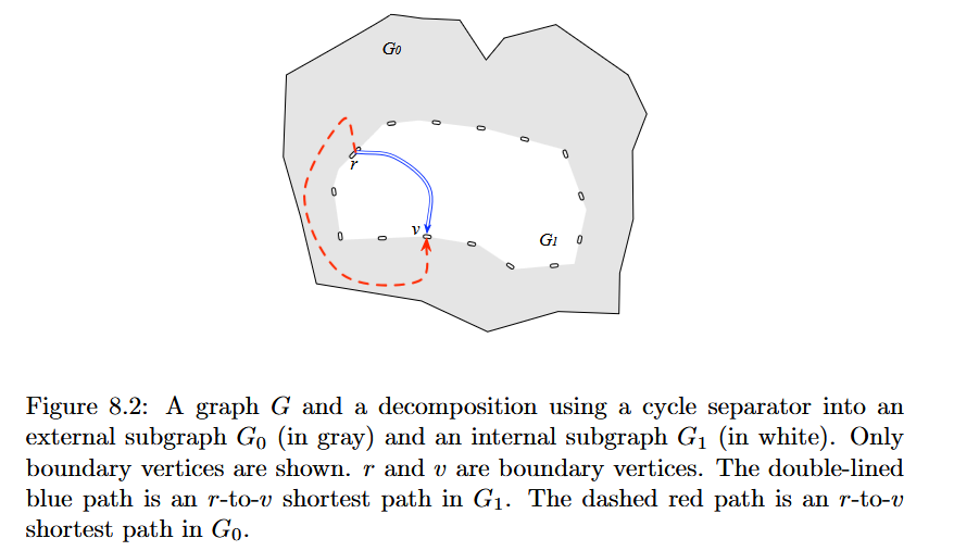
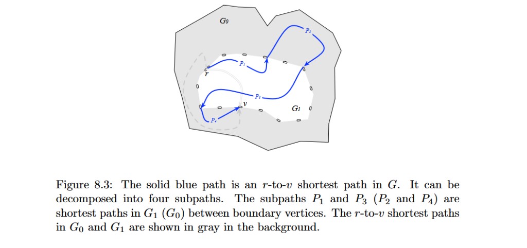
<p>And actually this is possible because we have the information of paths and distances implicitly stored in the distance subgraph, so for each boundary, to go into another boundary we must traverse different pieces from boundary to boundary, so running Dijkstra actually gives us the desired distances.</p>

<p><img src="/images/fr-klein-fig-8-2.png" alt="Klein Figure 8.2: cycle separator splitting G into an external subgraph G0 and an internal subgraph G1, with r-to-v shortest paths in each piece" style="max-width: 640px; height: auto; display: block; margin: 1.5em auto;" /></p>

<p><img src="/images/fr-klein-fig-8-3.png" alt="Klein Figure 8.3: an r-to-v shortest path in G decomposed into subpaths that alternate between G0 and G1, meeting only at boundary vertices" style="max-width: 640px; height: auto; display: block; margin: 1.5em auto;" /></p>

<p>Finally, for each piece \(P\), we attach an artificial source \(s'\) to each boundary vertex \(u\) with an edge of length</p>

\[d(s,u),\]

<p>where \(d(s,u)\) is the distance from \(s\) to \(u\) computed in the dense distance graph. We then compute a shortest-path tree in \(P\) rooted at \(s'\) using Dijkstra’s algorithm. Since each piece contains \(O(r)\) vertices, this takes</p>

\[O(r\log r)\]

<p>time per piece, or</p>

\[O\left(\frac{n}{r}\cdot r\log r\right) = O(n\log r)\]

<p>time overall.</p>

<p>Thus, the overall running time is</p>

\[O\left( n\log r + \frac{n}{\sqrt{r}}\log n + n \right).\]

<p>In particular, setting</p>

\[r=\Theta(\log^2 n)\]

<p>gives</p>

\[\log r=\Theta(\log\log n)\]

<p>and</p>

\[\frac{n}{\sqrt{r}}\log n = \frac{n}{\log n}\log n = O(n).\]

<p>Therefore, the total running time is</p>

\[O(n\log\log n).\]

<p>So as you can see, we incorporated terse sparsified local structures and their information to traverse the graph in a more efficient manner, then when we come sufficiently close, we can consider a piece or region with all of its nodes.</p>

<p>So now here come the ideas of the paper actually.
We want to use Dijkstra and Bellman–Ford in case we have negative cases eventually, but we want to do it in a more efficient manner. And one of the more useful techniques of doing so is to bypass the \(O(m)\) complexity of the relaxation phase for each vertex. And to do so, we must use some characteristics of planar graphs. And we will see how we can do it, do kind of bring it down to something like \(O(log(m))\). It’s a rough idea, and so in order to do that we must use the idea of a Monge array, that lets us to do a search like binary search.</p>

<p>A matrix \(M=(M_{ij})\) is <em>totally monotone</em> if for every \(i,i',j,j'\) such that \(i&lt;i'\) and \(j&lt;j'\), if</p>

\[M_{ij}\le M_{ij'},\]

<p>then</p>

\[M_{i'j}\le M_{i'j'}.\]

<p>A matrix \(M=(M_{ij})\) is <em>convex Monge</em> (respectively, <em>concave Monge</em>) if for every \(i,i',j,j'\) such that \(i&lt;i'\) and \(j&lt;j'\), we have</p>

\[M_{ij}+M_{i'j'} \ge M_{ij'}+M_{i'j}\]

<p>(respectively,</p>

<p>\(M_{ij}+M_{i'j'} \le M_{ij'}+M_{i'j}.\))</p>

<p>It is immediate that if \(M\) is convex Monge, then it is totally monotone. It is also easy to see that the matrix obtained by transposing \(M\) is also totally monotone.</p>

<p><strong>Remark.</strong> In 1987, Alok Aggarwal, Maria Klawe, Shlomo Moran, Peter Shor, and Robert Wilber described an elegant recursive algorithm that finds the minimum element in every row of an \(n\times n\) Monge array in \(O(n)\) time, now usually called the <em>SMAWK algorithm</em>.</p>

<p><strong>Theorem.</strong>
For any four indices \(k,k',\ell,\ell'\) such that either \(A_{k\ell}\), \(A_{k\ell'}\), \(A_{k'\ell}\), and \(A_{k'\ell'}\) are all in \(A\)’s upper triangle, or are all in \(A\)’s lower triangle (i.e., either</p>

\[1\le k\le k'\le \ell\le \ell'\le |V_c|\]

<p>or</p>

\[1\le \ell\le \ell'\le k\le k'\le |V_c|,\]

<p>the convex Monge property holds:</p>

\[A_{k\ell}+A_{k'\ell'} \ge A_{k\ell'}+A_{k'\ell}.\]
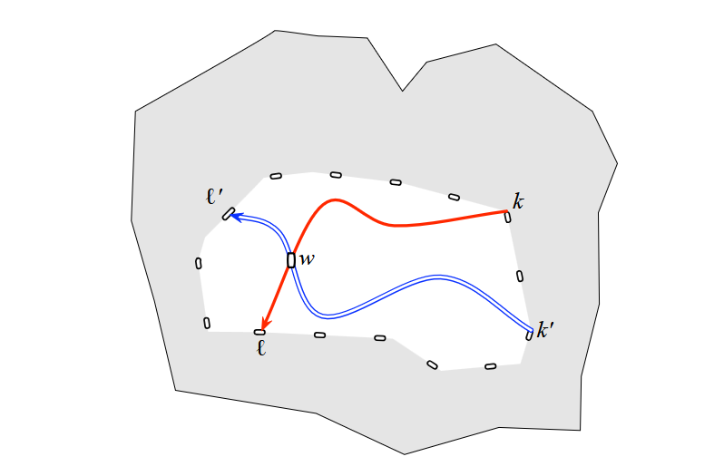
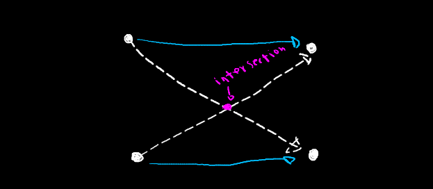
<p><img src="/images/fr-crossing-w.png" alt="Crossing shortest paths in a piece meeting at an intersection node w" style="max-width: 640px; height: auto; display: block; margin: 1.5em auto;" /></p>

<p><img src="/images/fr-uncrossing.png" alt="Uncrossing two paths at their intersection to derive the Monge inequality" style="max-width: 520px; height: auto; display: block; margin: 1.5em auto;" /></p>

<p><strong>Proof.</strong> It is simply a case of using the Jordan curve theorem, finding a middle node or intersection node and uncrossing the nodes to derive the inequality.</p>

<p>The Monge property also implies another important property that we use.
That is, for \(y\in B\), if \(u\in A\) is the node that minimizes \(d(u,y)\), then for any \(v\neq u\in A\) and \(x\neq y\in B\),</p>

\[d(v,x)\ge d(u,x).\]

<p>Given \((A,B,d)\) with the Monge property, the <em>Monge matching problem</em> is to find a parent \(p(v)\in A\) for all \(v\in B\) such that</p>

\[d(p(v),v)\le d(u,v) \qquad\text{for any }u\in A.\]

<p>The set of pairs</p>

\[\{(p(v),v):v\in B\}\]

<p>forms the <em>minimum Monge matching</em>.</p>

<p>The non-crossing property states that it is enough to look for a function \(p(\cdot)\) that has no “crossing.” Therefore, we can use standard divide-and-conquer techniques to derive an</p>

\[O(n\log n)\]

<p>algorithm for the problem, where</p>

\[n=|A|+|B|.\]

<p>Or constructively we can start from a row to find the min element in the column and use a binary search to add a row, and compute the local minima, which takes the same complexity and is basically the same algorithm.</p>

<p>so ok.</p>

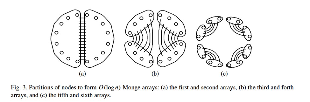
<p>General complete graphs are not Monge. We can preserve the information that the dense distance graph gives us using \(O(\log n)\) Monge arrays, by halving the cycle separator in half and considering only the distances between the two halves and continuing to do this recursively. This way we have at most \(O(\log n)\) levels of Monge matrix, which we can find the possible relaxation candidates simultaneously in \(O(k\log k)\) for which \(k\) is the number of rows and columns in one of the Monge arrays.</p>

<p><img src="/images/fr-monge-arrays.png" alt="Fakcharoenphol–Rao Fig. 3: recursive partitions of boundary nodes into O(log n) Monge arrays" style="max-width: 700px; height: auto; display: block; margin: 1.5em auto;" /></p>

<p><strong>Citing the paper.</strong></p>

<p>We accomplish this by maintaining the edges of each subpiece of \(P\) in \(O(\log n)\) levels of Monge arrays. After the definition of the Monge arrays, we describe how all edges in each Monge array with \(k\) nodes can be relaxed in \(O(k\log k)\) time, where \(k\) is the number of nodes in the data structure.</p>

<p>The first Monge array that we define is formed as follows. Divide the border nodes in some subpiece into two halves, the first (or left) half in the circular order (with an arbitrary starting point) and the second (or right) half. Consider the set of edges in the dense distance graph that go from the left border nodes to the right ones. The edges obey the Monge property, since there is an underlying shortest path tree in which the corresponding paths do not cross.</p>

<p>Using the same left–right partitioning, we can define another Monge array with the direction of edges reversed (i.e., edges in the array go from the right border nodes to the left border nodes).</p>

<p>So, when we want to simulate Dijkstra’s algorithm or Bellman–Ford, we only perform the relaxation operations within these related \(O(\log n)\) data structures.</p>

<p>Therefore, relaxing the edges can be done in</p>

\[O(\sqrt{n}\log^2 n),\]

<p>since the total number of nodes in all the data structures is</p>

\[O(\sqrt{n}\log n)\]

<p>for each subpiece of \(P\) in the decomposition, and relaxing the edges within a Monge array with \(k\) nodes takes \(O(k\log k)\) time.</p>

<p>In this way, we are handling the information in a very clever manner in order to obtain a better query or time complexity.</p>

<p>Suppose that we have no negative edge; for the other case we have to talk about Bellman–Ford too, which I probably won’t in this chapter or will later update this post.</p>

<p>So how does FR-Dijkstra work?</p>

<p>First of all we must know that things are computed in a clever data structure:</p>

<p><strong>On-line Bipartite Monge Search</strong></p>

<p>It is online in the sense that Dijkstra’s algorithm is online, because in each loop, after relaxation we can find a new node and set it to shortest distance instead of infinity.</p>

<p>An important subroutine in the efficient implementation of Dijkstra’s algorithm running on dense distance graphs is the <em>on-line bipartite Monge search</em> problem.</p>

<p>The algorithm computes shortest paths by combining several instances of the following problem.</p>

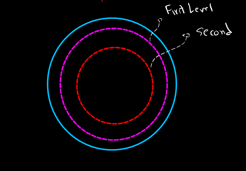
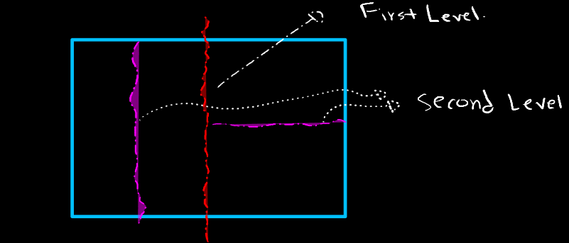
<p>Actually the way that we can recursively partition the graph has been improved since the time of the paper publication; they would halve the graph horizontally following the Tarjan–Lipton paper, but we can decompose the planar map cyclically in each step.</p>

<p><img src="/images/fr-nested-separators.png" alt="Cyclic nested separators: first level and second level inside a piece" style="max-width: 480px; height: auto; display: block; margin: 1.5em auto;" /></p>

<p><img src="/images/fr-recursive-levels.png" alt="Recursive separator levels: a first-level cut, then second-level cuts in each half" style="max-width: 520px; height: auto; display: block; margin: 1.5em auto;" /></p>

<p>So for each step we can compute the global to local structure of that piece, and we may at most do it \(\log n\) times, so the time complexity would be \(\log n\) times whatever complexity that we get.</p>

<p>And we recursively perform the algorithm that beat Dijkstra recursively to get from one layer to another layer of \(s\)–\(v\) shortest path.</p>

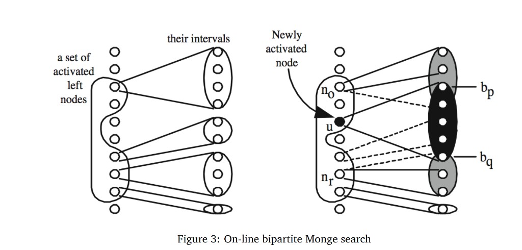
<p><strong>On-line bipartite Monge search.</strong>
Given \(d(x,y)\), representing a dense distance graph for \(X\times Y\), maintain a parent \(x\in X\) for every \(y\in Y\), while the initialization value \(D(\cdot)\) for each \(x\in X\) is revealed on-line, one node at a time.</p>

<p><img src="/images/fr-online-bipartite-monge.png" alt="On-line bipartite Monge search: activated left nodes and the intervals of Y they currently parent" style="max-width: 700px; height: auto; display: block; margin: 1.5em auto;" /></p>

<p>The matching can be computed on-line in overall time</p>

\[O\bigl((|X|+|Y|)\log(|X|+|Y|)\bigr),\]

<p>which is the same asymptotic time as the standard divide-and-conquer algorithm.</p>

<p>Maintaining a matching means, in this context, managing:</p>

<ul>
  <li>a set of active nodes \(A\subseteq X\); and</li>
  <li>a growing set of matched nodes \(M\subseteq Y\), or, more importantly, a shrinking set of yet-unmatched nodes \(Y\setminus M\).</li>
</ul>

<p>The data structure supports the following three operations, which are used by Dijkstra’s algorithm:</p>

<ul>
  <li><strong>FindMin()</strong>: returns the minimum unmatched node \(y\in Y\setminus M\). This functions as a priority queue for the right-hand side.</li>
  <li><strong>ExtractMin()</strong>: adds the current minimum node to \(M\).</li>
  <li><strong>ActivateLeft\((x,\delta)\)</strong>: reveals the initialization value \(D(x)=\delta\) for some \(x\in X\) and updates the preliminary matches.</li>
</ul>

<p><strong>Efficient Implementation.</strong></p>

<p>We use a heap and intervals in an ordered set \(Y\). Assume that, for each \(x\in X\), we have precomputed, together with the dense distance graph, a data structure supporting queries of the form</p>

\[\min_{i^-\le i\le i^+} d(x,y_i)\]

<p>for any \(i^-,i^+\). Note that this data structure is independent of \(D(x)\), and the query can be answered using an LCA data structure in \(O(1)\) time.</p>

<p>Maintain a binary search tree for the active nodes \(x\in A\).</p>

<p>For every active \(x\in A\), maintain an interval</p>

\[[i^-(x),i^+(x))\]

<p>of children \(y\in Y\). Here, \(x\) is the current parent of \(y\), although this parent may change over time.</p>

<p>Maintain a priority queue (heap) containing, for every active \(x\in A\), its shortest edge to an unmatched node \(y\in Y\setminus M\).</p>

<ul>
  <li>
    <p><strong>FindMin()</strong> returns the minimum element of the heap in \(O(1)\) time.</p>
  </li>
  <li>
    <p><strong>ExtractMin()</strong> adds the current minimum to \(M\). Suppose the minimum is \(y_j\in Y\setminus M\) with parent \(x\in A\). We need to insert the second-shortest edge from \(x\) into the heap.</p>

    <p>Instead, create two dummy nodes \(x'\) and \(x''\) spanning the intervals</p>

\[[i^-(x),j) \qquad\text{and}\qquad [j+1,i^+(x)),\]

    <p>respectively. Find the minimum in each of these intervals using the above LCA data structure for \(x\), and insert the resulting edges into the heap. This takes</p>

\[O(\log |Y|)\]

    <p>time.</p>

    <p>There are at most two new dummy nodes for each extracted node of \(Y\). Hence, there are only</p>

\[O(|X|+|Y|)\]

    <p>dummy nodes in total.</p>
  </li>
  <li>
    <p><strong>ActivateLeft\((x,\delta)\)</strong> activates a new node \(x\in X\) with initialization value</p>

\[D(x)=\delta.\]

    <p>First, compute its interval</p>

\[[i^-(x),i^+(x)).\]

    <p>If \(x\) is the first active node, the interval contains all of \(Y\). Otherwise, we proceed as follows.</p>

    <ol>
      <li>
        <p>Walk upward through the active nodes with non-empty intervals until reaching the first node \(x'\) such that</p>

\[d(x',y_{i^-(x')}) &lt; d(x,y_{i^-(x')}).\]

        <p>Then perform a binary search for \(i^-(x)\) in the range</p>

\[[i^-(x'),i^+(x')).\]

        <p>This takes</p>

\[O(\log |Y|)\]

        <p>time.</p>
      </li>
      <li>
        <p>Analogously, walk downward through the active nodes with non-empty intervals until reaching the first node \(x''\) such that</p>

\[d(x'',y_{i^+(x'')-1}) &lt; d(x,y_{i^+(x'')-1}).\]

        <p>Then perform a binary search for \(i^+(x)\) in the range</p>

\[[i^-(x''),i^+(x'')).\]

        <p>This also takes</p>

\[O(\log |Y|)\]

        <p>time.</p>
      </li>
    </ol>

    <p>Finally, update the other intervals and the heap.</p>

    <p>For nodes in \(A\) between \(x\) and \(x'\) (and between \(x\) and \(x''\)), the corresponding interval becomes empty. These nodes are therefore deactivated, and their corresponding minimum unmatched nodes in \(Y\setminus M\) are removed from the heap.</p>

    <p>Since the sequential search (the “walk up/down”) visits each such node at most once, its total cost is amortized</p>

\[O(\log |Y|)\]

    <p>per \(x\in X\).</p>

    <p>For \(x'\) and \(x''\), their intervals may shrink to</p>

\[[i^-(x'),i^-(x)) \qquad\text{and}\qquad [i^+(x)+1,i^+(x'')),\]

    <p>respectively. Either interval may also become empty. The corresponding minimum unmatched node in \(Y\setminus M\) is then updated in the heap, taking</p>

\[O(\log |Y|)\]

    <p>time.</p>
  </li>
</ul>

<p>So really we are keeping a global heap, local heaps for each half of the complete dense graph pieces, making them Monge. And the magic really happens when we are maintaining the parents for the right side of bipartite graphs, which takes \(\log Y\) times amortized. And the algorithm is true because just like the usual Dijkstra it is picking the edges greedily, so only we are using the structure to relax more efficiently.</p>

<p>And the real magic happens when we are handling the parents as I said, <strong>Reveal\((j,x)\)</strong> is implemented in \(O(\log k)\) amortized time as follows:</p>

<ul>
  <li>
    <p>Find the live intervals</p>

\[I^-=(j^-,i^-_{\min},i^-_{\min}) \qquad\text{and}\qquad I^+=(j^+,i^+_{\min},i^+_{\min})\]

    <p>immediately before and after \((j,\cdot,\cdot)\) in lexicographic order, in \(O(\log k)\) time, by querying the balanced binary search tree.</p>
  </li>
  <li>
    <p>While</p>

\[M[i^-_{\min},j] &lt; M[i^-_{\min},j^-],\]

    <p>replace \(I^-\) with its predecessor in lexicographic order. Then binary search for the smallest index \(i_{\min}\) such that</p>

\[M[i_{\min},j] &lt; M[i_{\min},j^-].\]
  </li>
  <li>
    <p>While</p>

\[M[i^+_{\min},j] &lt; M[i^+_{\min},j^+],\]

    <p>replace \(I^+\) with its successor in lexicographic order. Then binary search for the smallest index \(i_{\max}\) such that</p>

\[M[i_{\max},j] &lt; M[i_{\min},j^+].\]
  </li>
  <li>
    <p>Delete any live intervals \((j^\pm,\cdot,\cdot)\) that overlap</p>

\[(j,i_{\min},i_{\max})\]

    <p>from the priority queue.</p>
  </li>
  <li>
    <p>Insert the new live intervals</p>

\[(j,i_{\min},i_{\max}), \qquad (j^-,\cdot,i_{\min}-1), \qquad (j^+,i_{\max}+1,\cdot)\]

    <p>into the priority queue.</p>
  </li>
</ul>

<p>To obtain the claimed \(O(\log k)\) amortized time bound, we charge the time required to delete any interval from the priority queue to its earlier insertion. The requirement that we only hide rows when their minimum elements are visible implies that there is exactly one live interval in the revealed column.</p>

<p><strong>FR-Dijkstra\((G,s)\)</strong></p>

<div class="language-plaintext highlighter-rouge"><div class="highlight"><pre class="highlight"><code>for all v in V(G):
    d(v) ← ∞
d(s) ← 0
S ← ∅

Convert each DDG into bipartite DDGs (X_i, Y_i).

for each (X, Y) such that s ∈ Y:
    (X, Y).Insert(s, 0)
    Global.DecreaseKey((X, Y), 0)

while S ≠ V(G):
    (X, Y) ← Global.ExtractMin()
    u ← (X, Y).ExtractMin(Y \ M)

    if u ∉ S:
        for each (X', Y') such that u ∈ X':
            (X', Y').ActivateLeft(u, d(u))
            v ← (X', Y').FindMin(Y' \ M')
            Global.DecreaseKey((X', Y'), d(v))
        S ← S ∪ {u}

    v ← (X, Y).FindMin(Y \ M)
    Global.DecreaseKey((X, Y), d(v))
</code></pre></div></div>

<h2 id="sources">Sources</h2>

<ul>
  <li>Jittat Fakcharoenphol and Satish Rao, <em>Planar graphs, negative weight edges, shortest paths, and near linear time</em>. <a href="https://doi.org/10.1016/j.jcss.2005.05.007">Journal of Computer and System Sciences</a> (the 2006 paper this post is about).</li>
  <li>Erik Demaine, MIT 6.889, Lecture 12: <a href="https://courses.csail.mit.edu/6.889/fall11/lectures/L12.pdf">Multiple-Source Shortest Paths</a>.</li>
  <li>Philip Klein, <a href="https://planarity.org/Klein_shortest_paths_with_negative_lengths.pdf"><em>Shortest paths in planar graphs with negative lengths</em></a>.</li>
  <li>Jeff Erickson, computational topology notes: <a href="https://jeffe.cs.illinois.edu/teaching/comptop/2023/notes/15-shortest-paths.pdf">15 — Shortest paths</a> and <a href="https://jeffe.cs.illinois.edu/teaching/comptop/2023/notes/17-faster-minimum-cut.pdf">17 — Faster minimum cut</a>.</li>
</ul>]]></content><author><name>Taha</name><email>tahahoseinpourasli@gmail.com</email></author><category term="planar graphs" /><category term="shortest paths" /><category term="FR-Dijkstra" /><category term="Monge arrays" /><category term="r-division" /><summary type="html"><![CDATA[Notes on Fakcharoenphol–Rao (2006): r-divisions, the dense distance graph, Monge arrays, and FR-Dijkstra on planar maps.]]></summary></entry><entry><title type="html">Dynamic Approximate Nearest-Neighbor Search in Doubling Metrics</title><link href="https://thomasgraceman.github.io/posts/dynamic-approximate-nns/" rel="alternate" type="text/html" title="Dynamic Approximate Nearest-Neighbor Search in Doubling Metrics" /><published>2026-08-06T00:00:00+00:00</published><updated>2026-08-06T00:00:00+00:00</updated><id>https://thomasgraceman.github.io/posts/DD</id><content type="html" xml:base="https://thomasgraceman.github.io/posts/dynamic-approximate-nns/"><![CDATA[<p>Well, in this blog post we are going to review several papers and understand the techniques that are utilized in order to tackle several problems related to areas such as nearest neighbor problems, the facility location problem, and so on.</p>

<p>I am going to study and explain three papers which have led to a dynamic solution for the facility location problem.</p>

<p>Ok, I think in the series of the several papers that I am going to review, the data structure designed by James Lee and his co-author is a revealing piece.</p>

<p>Nearest-neighbor search (NNS) is the problem of preprocessing a set $S$ of $n$ points lying in a huge (possibly infinite) metric space $(M,d)$ so that, given a query $q \in M$, one can efficiently locate the nearest point to $q$ among the points in $S$.</p>

<p>Let $q$ be the query and $a \in S$ the closest point to $q$ in $S$. Then a $(1+\varepsilon)$-NNS algorithm is one which, given $q$, returns some $s \in S$ such that</p>

\[d(q,s) \leq (1+\varepsilon)\, d(q,a).\]

<p>So while it is NP-hard to return the nearest neighbor, it is worthwhile to examine whether we can approximate the answer in an efficient manner. Lee and his co-author used a very interesting classic idea: move from coarse to fine approximation. In a sense, their data structure is analogous to the binary search algorithm, with an extra twist and turn. Moreover, they employ the idea of doubling dimension as a means to count the complexity of the algorithm that they propose.</p>

<p>The doubling dimension of a metric space $(X,d)$, denoted in this post by $\dim(X)$, is the minimum value $\rho$ such that every set in $X$ can be covered by $2^{\rho}$ sets of half the diameter. (The diameter of a set $S \subseteq X$ is</p>

\[\sup\{\,d(x,y) : x,y \in S\,\}.\]

<p>)</p>

<p>A metric space is called <em>doubling</em> if its doubling dimension is $O(1)$. This notion of dimension measures the “volume growth” of $X$.</p>

<p>So, following the paper, we want to prove the following result:</p>

<p><strong>Theorem.</strong> Let $(S,d)$ be a finite metric space with doubling dimension $\dim(S)$ and aspect ratio $\Delta=\Delta_S$, defined as</p>

\[\Delta_S = \frac{\displaystyle\max_{x,y\in S} d(x,y)}{\displaystyle\min_{\substack{x,y\in S\\x\neq y}} d(x,y)}.\]

<p>Then there exists a dynamic data structure for approximate nearest-neighbor search with the following properties:</p>

<ol>
  <li>The data structure uses $O(n)$ space if $S$ is doubling.</li>
  <li>It answers $(1+\varepsilon)$-nearest-neighbor queries in</li>
</ol>

\[O(\log \Delta)+\left(\frac{1}{\varepsilon}\right)^{O(1)}\]

<p>time.</p>
<ol>
  <li>It supports insertions and deletions in</li>
</ol>

\[O(\log \Delta\,\log\log \Delta)\]

<p>time.</p>

<p>Moreover, in most applications,</p>

\[\Delta=\operatorname{poly}(|S|),\]

<p>and therefore</p>

\[\log\Delta=O(\log n).\]

<p>The running time depends exponentially on $\dim(S)$. Furthermore, in the distance-oracle model, where access to the ambient metric space is restricted to distance queries, this exponential dependence on the doubling dimension is necessary.</p>

<p>So let us first follow a simplified version of the data structure.</p>

<p>Let $(S,d)$ be the metric space against which queries are performed. For the sake of this informal discussion, assume that the minimum interpoint distance in $S$ satisfies</p>

\[\min\{d(x,y): x,y\in S,\ x\neq y\}=1.\]

<p>Under this assumption, the aspect ratio $\Delta$ is simply the diameter of $S$.</p>

<p>In what follows, for a subset $R\subseteq S$ and a point $x\in M$, we define</p>

\[d(x,R)=\inf_{y\in R} d(x,y).\]

<p>Let $k=\log \Delta$, and for each $i=0,1,\ldots,k$, let $Y_i$ be a $2^i$-net of $S$. For every point $y\in Y_i$, define the set</p>

\[L_{y,i} = \left\{ z\in Y_{i-1} : d(y,z)\leq \gamma 2^i \right\},\]

<p>where $\gamma$ is a constant to be specified later.</p>

<p>So what are we going to do here? We are providing details from coarse to fine for the underlying data structure! And $L_{y,i}$ gives us a means to search through the metric space. I would rather call them approximate $2^{i-1}$ neighbors of the given point. So we have a means of sparsifying the metric space, and we build a tree based on the sparsification. It is obvious that we can build the nets in a greedy manner.</p>

<p>Since $L_{y,i}\subseteq Y_{i-1}$, and $Y_{i-1}$ is a $2^{i-1}$-net, any two distinct points of $L_{y,i}$ satisfy</p>

\[d(z_1,z_2)\ge 2^{i-1}, \qquad \forall\, z_1\neq z_2\in L_{y,i}.\]

<p>Hence, the minimum interpoint distance in $L_{y,i}$ is $2^{i-1}$.</p>

<p>Moreover, by the definition</p>

\[L_{y,i} = \{z\in Y_{i-1}: d(y,z)\le \gamma 2^i\},\]

<p>every point of $L_{y,i}$ lies within distance $\gamma 2^i$ of the center $y$. Therefore, for any $z_1,z_2\in L_{y,i}$, the triangle inequality gives</p>

\[d(z_1,z_2) \le d(z_1,y)+d(y,z_2) \le \gamma 2^i+\gamma 2^i = \gamma 2^{i+1}.\]

<p>Thus,</p>

\[\operatorname{diam}(L_{y,i}) \le \gamma 2^{i+1}.\]

<p>Consequently, the aspect ratio of $L_{y,i}$ is bounded by</p>

\[\frac{\operatorname{diam}(L_{y,i})}{\min\{d(z_1,z_2):z_1\neq z_2,\ z_1,z_2\in L_{y,i}\}} \le \frac{\gamma 2^{i+1}}{2^{i-1}} = 4\gamma,\]

<p>which is a constant.</p>

<p>So, in order to count the number of children of any node in the tree, we use the doubling property and use that to count the number of children.</p>

<p><strong>Lemma.</strong> Let $(S,d)$ be a metric space, and let $Y\subseteq S$. If the aspect ratio of the metric induced on $Y$ is at most $\alpha$, where $\alpha\ge 2$, then</p>

\[|Y|\le \alpha^{O(\dim(S))}.\]

<p><em>Proof.</em> Let</p>

\[d_{\min} = \inf\{d(x,y):x,y\in Y,\ x\neq y\}\]

<p>and</p>

\[d_{\max} = \sup\{d(x,y):x,y\in Y\}\]

<p>be the minimum and maximum interpoint distances in $Y$, respectively. Assume that</p>

\[\alpha=\frac{d_{\max}}{d_{\min}}&lt;\infty.\]

<p>Notice that $Y$ is contained in a ball of radius</p>

\[2d_{\max}\le 2\alpha d_{\min},\]

<p>centered at any point of $Y$.</p>

<p>Applying the definition of doubling dimension iteratively, this ball (and hence $Y$) can be covered by</p>

\[2^{\dim(S)\cdot O(\log\alpha)}\]

<p>balls of radius</p>

\[\frac{d_{\min}}{3}.\]

<p>Each such ball can contain at most one point of $Y$. Indeed, if two distinct points of $Y$ were contained in the same ball, then by the triangle inequality their distance would be at most</p>

\[2\cdot\frac{d_{\min}}{3} = \frac{2d_{\min}}{3} &lt; d_{\min},\]

<p>contradicting the definition of $d_{\min}$.</p>

<p>Therefore,</p>

\[|Y| \le 2^{\dim(S)\cdot O(\log\alpha)} = \alpha^{O(\dim(S))}.\]

<p>When $S$ is a doubling metric, the Lemma implies that</p>

\[|L_{y,i}|=O(1),\]

<p>where the hidden constant depends only on the choice of $\gamma$ (and the doubling dimension of $S$).</p>

<p>Furthermore, the top-level net $Y_k$ contains exactly one (arbitrary) point, which we denote by</p>

\[y_{\mathrm{top}}.\]

<p>Given a query point $q\in M$, we first set</p>

\[y=y_{\mathrm{top}}.\]

<p>Then, iteratively for</p>

\[i=k,k-1,\ldots,1,\]

<p>we find the point in</p>

\[L_{y,i}\subseteq Y_{i-1}\]

<p>that is closest to $q$, and update $y$ to be this point for the next iteration.</p>

<p>If, at some stage, we reach a point such that</p>

\[d(q,L_{y,i})&gt;3\cdot 2^{i-1},\]

<p>then we stop the procedure and output the current value of $y$. Otherwise, after completing all iterations, we output the final value</p>

\[y\in Y_0.\]

<p>First, notice that the running time of this algorithm is at most</p>

\[O(\log \Delta),\]

<p>since finding the closest point to $q$ among a list $L_{y,i}$ takes constant time. This follows from the fact that every list has size</p>

\[|L_{y,i}|=O(1).\]

<p>It remains only to prove that the output point $y$ is a $3$-approximation to the nearest neighbor. Let $a\in S$ be the true nearest neighbor of $q$. We need to show that</p>

\[d(q,y)\leq 3d(q,a).\]

<p>To this end, let $j$ be such that</p>

\[d(q,y)\leq 3\cdot 2^j,\]

<p>but</p>

\[d(q,L_{y,j})&gt;3\cdot 2^{j-1},\]

<p>i.e., the step in which the distance does not decrease by a factor of $2$. Since the closest $2^{j-1}$-net point to $a$ satisfies</p>

\[d(a,L_{y,j})\leq 2^{j-1},\]

<p>the closest $2^{j-1}$-net point to $a$ is contained in $L_{y,j}$. Let $y^*\in Y_{j-1}$ be such that</p>

\[d(a,y^*)\leq 2^{j-1}.\]

<p>We need to show that</p>

\[d(y^*,y)\leq \gamma 2^j.\]

<p>In this case, we have $y^*\in L_{y,j}$. Using the triangle inequality,</p>

\[\begin{aligned}
d(y^*,y) &amp;\leq d(y^*,a)+d(a,y)\\
&amp;\leq 2^{j-1}+d(a,q)+d(q,y)\\
&amp;\leq 2^{j-1}+2d(q,y)\\
&amp;\leq 7\cdot 2^j .
\end{aligned}\]

<p>Therefore, choosing</p>

\[\gamma=7\]

<p>suffices.</p>

<p>This shows that the descent process “tracks” the closest net point to $a$. Now, we have</p>

\[3\cdot 2^{j-1} &lt; d(q,L_{y,j}) \leq d(q,a)+d(a,L_{y,j}) \leq d(q,a)+2^{j-1}.\]

<p>Hence,</p>

\[d(q,a)&gt;2^j.\]

<p>Since</p>

\[d(q,y)\leq 3\cdot 2^j,\]

<p>we conclude that</p>

\[d(q,y)\leq 3d(q,a).\]

<p>Therefore, $y$ is a $3$-approximate nearest neighbor of $q$.</p>

<p>Similar arguments show that if the algorithm terminates with</p>

\[y\in Y_0,\]

<p>then $y$ is actually the closest point to $q$ in $S$, because we have a $1$-net and we have the closest point to $a$ in the set $L_{y,i}$.</p>

<p>For a technical reason, the above data structure does not support efficient deletions and might require space</p>

\[\Omega(n\log\Delta).\]

<p>The main remedy for these latter problems is to choose $Y_i$ to be a $2^i$-net of $Y_{i-1}$ rather than a $2^i$-net of $S$.</p>

<p>Let us get into the main algorithm.</p>

<p>Let</p>

\[\Gamma=\{2^i:i\in\mathbb{Z}\},\]

<p>and call every value $r\in\Gamma$ a <em>scale</em>. Only $O(\log\Delta)$ of these scales are relevant; the remaining scales are trivial.</p>

<p>For every $r\in\Gamma$, let $Y_r$ be an $r$-net of $Y_{r/2}$. We define</p>

\[Y_r:=S\]

<p>for all scales</p>

\[r\leq d_{\min}.\]

<p>For every $r\in\Gamma$ and every $y\in Y_r$, …</p>

<p>so we are making the details more coarse by only having the nets in $Y_i$ instead of $S$.</p>

<p>For every $r\in\Gamma$ and every $y\in Y_r$, the data structure stores a list of the nearby points to $y$ among the $(r/2)$-net $Y_{r/2}$. This scale-$r$ navigation list of $y$ is defined as</p>

\[L_{y,r} := \left\{ z\in Y_{r/2}: d(z,y)\leq \gamma r \right\},\]

<p>where $\gamma&gt;0$ is a universal constant.</p>

<p>So we are roughly halving the distance at each step.</p>

<p><strong>Lemma.</strong> For every scale $r$, the following properties hold:</p>

<ol>
  <li>
    <p><strong>Covering:</strong>
\(d(z,Y_r)&lt;2r\)
for every $z\in S$.</p>
  </li>
  <li>
    <p><strong>Packing:</strong>
\(d(x,y)\geq r\)
for every $x,y\in Y_r$ with $x\neq y$.</p>
  </li>
</ol>

<p>The proofs are easy, and the first one follows by induction. So, it adheres to our intuition of having a rougher estimation while also helping us to preserve space in our algorithm.</p>

<p>We also have the following lemma.</p>

<p><strong>Lemma.</strong> The size of every navigation list is at most</p>

\[2^{O(\dim(S))}.\]

<p>which has the same proof as before.</p>

<p>The data structure maintains this point $y_{\mathrm{top}}$ and the cutoff scale</p>

\[r_{\max} := \min\{r\in\Gamma:\forall r'\geq r,\ |Y_{r'}|=1\},\]

<p>for the sake of bootstrapping most of the operations.</p>

<p>Third, for all scales</p>

\[r\leq d_{\min},\]

<p>the net $Y_r$ is equal to $S$. Therefore, for scales</p>

\[r\leq d_{\min}/2,\]

<p>every point $x\in S$ has a trivial list</p>

\[L_{x,r}=\{x\}.\]

<p>These trivial lists can be represented succinctly by storing, for every $x\in S$, a scale $r_x\in\Gamma$ below which all lists of $x$ are trivial. For the sake of analysis, define</p>

\[r_{\min}:=\min\{r_x:x\in S\}.\]

<p><strong>Lemma.</strong> The cutoff scales satisfy</p>

\[r_{\max}=\Theta(d_{\max})\]

<p>and</p>

\[r_{\min}=\Theta(d_{\min}).\]

<p>Consequently, every point has</p>

\[O(\log\Delta)\]

<p>non-trivial navigation lists.</p>

<p>The proof is easy.</p>

<p>Combining the above results, we obtain an upper bound on the total space required by the data structure. Specifically, the space complexity is</p>

\[n\cdot 2^{O(\dim(X))}\log\Delta .\]

<p>For each point $x\in S$, the non-trivial navigation lists of $x$ are stored using, for example, a balanced search tree. This requires linear space and supports the operations find, insert, and delete in logarithmic time.</p>

<p>It then follows from Lemma 2.3 that inserting a new navigation list for a point can be performed in time</p>

\[O(\log\log\Delta).\]

<p><strong>Theorem.</strong> The size of the data structure is</p>

\[2^{O(\dim(S))}\cdot n\]

<p>words.</p>

<p><em>Proof.</em> The proof bounds the size using a charging argument.</p>

<p><strong>Definition.</strong> A subset $Z_r\subseteq Y_r$ is called <em>non-proper</em> if it contains only one point $x$ and</p>

\[r_x&gt;r.\]

<p>Otherwise, $Z_r$ is called <em>proper</em>.</p>

<p><strong>Algorithm: Approx-NNS</strong></p>

<p><em>Input:</em> $q\in X$ and $\varepsilon&gt;0$.</p>

<ol>
  <li>Set</li>
</ol>

\[r=r_{\max}\]

<p>and</p>

\[Z_r=\{y_{\mathrm{top}}\}.\]

<ol>
  <li>While</li>
</ol>

\[2r\left(1+\frac{1}{\varepsilon}\right)&gt;d(q,Z_r)\]

<p>and $Z_r$ is proper, do:</p>

<p>a. Set</p>

\[Z_{r/2} = \left\{ y\in \bigcup_{z\in Z_r}L_{z,r} : d(q,y)\leq d(q,Z_r)+r \right\}.\]

<p>b. Set</p>

\[r=r/2.\]

<ol>
  <li>Return the point $z\in Z_r$ for which</li>
</ol>

\[d(q,z)\]

<p>is minimal.</p>

<p><strong>Lemma.</strong> Let $a$ be a closest point to $q$ among $S$. Then every set $Z_r$ computed by Procedure Approx-NNS contains a point $z_r$ such that</p>

\[d(a,z_r)\leq 2r.\]

<p><strong>Lemma.</strong> Procedure Approx-NNS outputs a point whose distance from $q$ is at most</p>

\[(1+\varepsilon)d(q,S).\]

<p><em>Proof.</em> Let $r^*$ be the value of $r$ at the end of the procedure. It suffices to prove that</p>

\[d(q,Z_{r^*})\leq (1+\varepsilon)d(q,S),\]

<p>because then the proof follows from the choice made in line 5 of the procedure.</p>

<p>There are two conditions in line 2 that may cause the while-loop to terminate. First, consider the case where</p>

\[2r^*\left(1+\frac{1}{\varepsilon}\right) \leq d(q,Z_{r^*}).\]

<p>By the previous lemma, we know that</p>

\[d(q,Z_{r^*})\leq d(q,S)+2r^*.\]

<p>Combining the above inequalities, we obtain</p>

\[\frac{2r^*}{\varepsilon}\leq d(q,S).\]

<p>Substituting this bound back into the previous inequality gives</p>

\[d(q,Z_{r^*}) \leq d(q,S)+2r^* \leq (1+\varepsilon)d(q,S),\]

<p>as desired.</p>

<p>Consider now the case where $Z_{r^*}$ is non-proper. We may assume that</p>

\[d(q,Z_{r^*})&gt;0,\]

<p>otherwise the claim is immediate.</p>

<p>For analysis, suppose we continue the procedure without the condition that $Z_r$ is proper. This process must terminate, since</p>

\[d(q,Z_r)\geq d(q,S)&gt;0,\]

<p>while</p>

\[2r\left(1+\frac{1}{\varepsilon}\right)\rightarrow 0.\]

<p>Moreover, the returned point remains unchanged, because all further sets $Z_r$ for $r&lt;r^<em>$ contain the same single point as $Z_{r^</em>}$. It is easy to see that the above analysis (including Lemma 2.4) also applies to the modified procedure. Therefore, both the modified and the actual procedure satisfy</p>

\[d(q,Z_{r^*})\leq (1+\varepsilon)d(q,S).\]

<p>In fact, if the procedure stops with a non-proper set $Z_r$, then it returns the unique closest point to $q$ in $S$. This follows by applying the same modified-procedure argument with an arbitrarily small $\varepsilon&gt;0$.</p>

<p><strong>Lemma.</strong> Procedure Approx-NNS runs in time</p>

\[2^{O(\dim(S))}\log\Delta + (1/\varepsilon)^{O(\dim(S))}.\]

<p><em>Proof.</em> Since the distance between any two points of</p>

\[Z_{r/2}\subseteq Y_{r/2}\]

<p>is at least $r/2$, Lemma 1.2 implies that</p>

\[|Z_{r/2}| \leq (2+1/\varepsilon)^{O(\dim(S))}.\]

<p>A simpler bound is obtained by separately bounding the number of iterations of the procedure and the running time of a single iteration. For the first part, consider the number of iterations performed by the procedure.</p>

<p><strong>Theorem.</strong> The data structure can be updated after inserting a point into $S$ in time</p>

\[2^{O(\dim(S))}\log\Delta\log\log\Delta .\]

<p>This update includes</p>

\[2^{O(\dim(S))}\log\Delta\]

<p>distance computations.</p>

<p><em>Proof sketch.</em> The main idea is that, regardless of how the nets were constructed, each $r$-net $Y_r$ can be updated after an insertion of a new point $q$ by either adding $q$ to $Y_r$ or leaving it unchanged.</p>

<p>This follows by induction on the scale $r$. For the base case, consider a sufficiently small scale $r$. By definition, $Y_r$ contains all points of $S$, and therefore $q$ must be added to this net.</p>

<p>For the inductive step, first assume that the update to $Y_{r/2}$ leaves it unchanged. In this case, $Y_r$ also remains unchanged. Otherwise, suppose that $q$ is added to $Y_{r/2}$. We then update $Y_r$ by adding $q$ to it if and only if</p>

\[d(q,Y_r)\geq r.\]

<p>This guarantees that $Y_r$ remains an $r$-net of $Y_{r/2}$ (although other valid updates are also possible).</p>

<p>To decide whether</p>

\[d(q,Y_r)\geq r,\]

<p>we use a set $Z_r$ that contains all points of $Y_r$ that are sufficiently close to $q$.</p>

<p>Recall that the net $Y_r$ is maintained only through its navigation lists. Therefore, adding $q$ to $Y_r$ requires constructing the scale-$r$ navigation list of $q$ and updating the scale-$2r$ navigation lists of nearby points. Both tasks are performed using the sets $Z_r$.</p>

<p>The proof uses induction on the scale $r$ to decide whether a new point $q$ should be added to the net $Y_r$.</p>

<p><strong>Base case (smallest scale).</strong> At the finest scale, $Y_r$ contains all points of $S$ by definition. Therefore, the new point $q$ must be added to $Y_r$.</p>

<p><strong>Inductive step.</strong> Assume that the update rule is correct for the smaller scale $r/2$. We consider two cases.</p>

<ol>
  <li><strong>$q$ is not added to $Y_{r/2}$.</strong></li>
</ol>

<p>In this case, $q$ is already within distance less than $r/2$ of some point in $Y_{r/2}$. Hence, it is also covered at scale $r$, and there is no need to add $q$ to $Y_r$.</p>

<ol>
  <li><strong>$q$ is added to $Y_{r/2}$.</strong></li>
</ol>

<p>Now we decide whether $q$ should also be added to $Y_r$. The condition is whether $q$ is sufficiently far from all existing points of $Y_r$:</p>

\[d(q,Y_r)\geq r.\]

<p>If this condition holds, we add $q$ to $Y_r$. Otherwise, $Y_r$ remains unchanged.</p>

<p>This update rule preserves the invariant that $Y_r$ is an $r$-net of $Y_{r/2}$.</p>

<p><strong>Step 3: Using $Z_r$ for efficient distance checks.</strong></p>

<p>A naive check of the condition</p>

\[d(q,Y_r)\geq r\]

<p>would require computing the distance from $q$ to every point in $Y_r$, which is too expensive.</p>

<p>Instead, the algorithm maintains a local set $Z_r$ that contains all points of $Y_r$ that are sufficiently close to $q$. Since $S$ has bounded doubling dimension $\dim(S)$, the number of points that can exist in such a local neighborhood while maintaining the packing property of the net is bounded by</p>

\[2^{O(\dim(S))}.\]

<p>Therefore, it is sufficient to check the distance between $q$ and the points in $Z_r$. If no point in $Z_r$ is within distance $r$ of $q$, then</p>

\[d(q,Y_r)\geq r,\]

<p>and we add $q$ to $Y_r$. Otherwise, $Y_r$ remains unchanged.</p>

<p><strong>Step 4: Updating the navigation lists.</strong></p>

<p>If $q$ is added to $Y_r$, the update of the data structure is not complete yet. The navigation lists, which connect points between consecutive scales, must also be updated.</p>

<p>First, we construct the scale-$r$ navigation list of $q$, which contains the nearby points of $q$ in the coarser net $Y_{2r}$.</p>

<p>Second, we update the scale-$2r$ navigation lists of all nearby points in $Y_{2r}$ by adding $q$ as one of their neighbors.</p>

<p>The set $Z_r$ is used to identify exactly the points whose navigation lists must be updated. Since $Z_r$ has size bounded by</p>

\[2^{O(\dim(S))},\]

<p>the update remains local and can be performed efficiently.</p>

<p>The final update time is</p>

\[2^{O(\dim(S))}\log\Delta\log\log\Delta .\]

<p>The complexity can be understood as follows.</p>

<p><strong>Local work.</strong> At each scale, the algorithm only examines the local set $Z_r$. By the doubling dimension bound,</p>

\[|Z_r|\leq 2^{O(\dim(S))}.\]

<p>Therefore, the distance computations and navigation-list updates performed at a single scale require</p>

\[2^{O(\dim(S))}\]

<p>time.</p>

<p><strong>Data structure overhead.</strong> The navigation lists are maintained using balanced search trees. Each insertion or update of a navigation list requires an additional</p>

\[O(\log\log\Delta)\]

<p>overhead. Therefore, the total update time is</p>

\[2^{O(\dim(S))} \cdot \log\Delta \cdot \log\log\Delta .\]

<p>Moreover, at each of the $O(\log\Delta)$ scales, the algorithm computes distances only to the</p>

\[2^{O(\dim(S))}\]

<p>points in the corresponding local set $Z_r$. Hence, the total number of distance computations is</p>

\[2^{O(\dim(S))}\log\Delta .\]

<p>And the scale is handled automatically by the insertion update.</p>

<h2 id="references">References</h2>

<ul>
  <li>R. Krauthgamer and J. R. Lee, <em>Navigating Nets: Simple Algorithms for Proximity Search</em>. In Proceedings of the Fifteenth Annual ACM-SIAM Symposium on Discrete Algorithms (SODA 2004), pp. 798–807. <a href="https://homes.cs.washington.edu/~jrl/papers/pdf/nn-soda.pdf">PDF</a></li>
</ul>]]></content><author><name>Taha</name><email>tahahoseinpourasli@gmail.com</email></author><category term="nearest neighbor search" /><category term="doubling dimension" /><category term="data structures" /><category term="metric spaces" /><summary type="html"><![CDATA[Study notes on a dynamic data structure for approximate nearest-neighbor search in doubling metrics.]]></summary></entry><entry><title type="html">Dynamic Sum-of-Radii Clustering</title><link href="https://thomasgraceman.github.io/posts/dynamic-sum-of-radii-clustering/" rel="alternate" type="text/html" title="Dynamic Sum-of-Radii Clustering" /><published>2026-08-06T00:00:00+00:00</published><updated>2026-08-06T00:00:00+00:00</updated><id>https://thomasgraceman.github.io/posts/Dynamic-Sum-of-Radii-Clustering</id><content type="html" xml:base="https://thomasgraceman.github.io/posts/dynamic-sum-of-radii-clustering/"><![CDATA[<p>So in this second post, following the <a href="/posts/dynamic-approximate-nns/">previous data structure</a>, I am going to review some algorithms that were devised using the scheme of nearest neighbor search.</p>

<p><strong>Definition (Dynamic Sum-of-Radii Clustering).</strong> They studied the dynamic sum-of-radii clustering problem, defined as follows. The original input consists of a (possibly infinite) set \(V\) of potential clients or points, a finite set \(F \subseteq V\) of facilities with an opening cost \(f_j\) for each facility \(j \in F\), and a metric \(d\) over \(V\).</p>

<p>For the online input, a set \(C\) of live clients evolves over time: at each timestep \(t\), either a new client arrives and is added to \(C\), or a client from \(C\) departs and is removed from \(C\), a query is made for the approximate cost of an optimal solution (<em>cost query</em>), or a query asks for the entire current solution (<em>solution query</em>).</p>

<p>For the output, at each timestep the algorithm maintains a set of open facilities, each open facility \(j\) being associated to a radius \(R_j\), such that every client of \(C\) is covered, i.e., belongs to some open ball \(B(j, R_j)\), and the goal is to minimize the cost, namely, the sum over open facilities \(j\) of \(f_j + R_j\).</p>

<p>The dynamic sum-of-radii clustering problem can actually be interpreted as a special case of dynamic set cover.</p>

<p>The doubling dimension of a metric space \((V, d)\) is said to be bounded by \(\kappa\) if any ball \(B(x, r)\) in \((V, d)\) can be covered by \(2^\kappa\) balls of radius \(r/2\), as defined in the previous post based on Lee’s paper.</p>

<p>The algorithm designed by them answers cost queries in constant time and solution queries in linear time in the size of the solution, up to a factor of \(\log(W/f_{\min})\), where \(W\) is the diameter of the metric space and \(f_{\min}\) is the minimum opening cost of any facility.</p>

<p><strong>Theorem.</strong> There exists an algorithm for the dynamic sum-of-radii clustering problem, when clients and facilities live in a metric space with doubling dimension \(\kappa\), such that at every timestep the solution has cost at most \(O(2^{2\kappa})\) times the cost of an optimal solution at that time, and such that the update time is \(O(2^{6\kappa} \log(W/f_{\min}))\), where \(W\) is the diameter of the space, \(n\) is the current number of clients, and \(f_{\min}\) is the minimum opening cost. A cost query can be answered in constant time, and a solution query in time \(O(s \log(W/f_{\min}))\), where \(s\) is the size of the output.</p>

<p>There exists a collection \(\Pi\) of pairs \(\langle j, r \rangle\) where \(j \in F\) and \(r\) is a non-negative integer, each with an associated area \(A(j, r)\) of \(V\), and an abstract tree \(T\) over \(\Pi\), with the following properties:</p>

<ol>
  <li>\(T\) has height \(O(\log(W/f_{\min}))\) and degree at most \(2^{4\kappa}\).</li>
  <li>The collection \(\mathcal{A}\) of areas is a laminar family, its laminar structure is given by \(T\), and for each area, \(A(j, r) \subseteq B(j, 7 \cdot 5^r)\).</li>
  <li>For any subset \(C\) of \(V\), there exists a collection \(S\) of areas covering \(C\) and whose cost,</li>
</ol>

\[\sum_{\langle j,r \rangle \in S} \left(f_j + 7 \cdot 5^r\right),\]

<p>is \(O(2^{2\kappa})\) times the optimal cost for \(C\).</p>

<p>So if you pay close attention, they are really using the scheme and the paradigm used by Lee and his co-author, really by maintaining a tree with nodes as a set of \(Z_{r/2}\) (namely, the points that are sufficiently close in the \(2^i\) net to the point that is being queried upon). But now the difficulty lies in the fact that we have to keep track of the opening cost, so we have to think of a heuristic there to come up with a good solution.</p>

<p>So the algorithm runs in two phases: one processes the data and finds a solution, and the other maintains the solution by the successive updates that come along the way. They start by discretizing a potential solution to the problem.</p>

<p><strong>Lemma.</strong> For all \(C \subseteq V\), there exists a solution such that every ball \(B(j, R)\) has \(f_{\min} \leq f_j \leq R \leq 5 \cdot W\), the radius \(R\) is an integer power of 5, and the cost is \(O(\text{OPT})\).</p>

<p><em>Proof.</em> Consider the unknown optimal solution. If some ball is such that \(\max(f_j, R) &gt; W\), then replace the entire solution by a ball centered at the facility of cost \(f_{\min}\) and of radius \(W\). Else, for each ball \(B(j, R)\) of the optimal solution:</p>

<ul>
  <li>if \(f_j &gt; R\) then increase the radius of the ball from \(R\) to \(f_j\).</li>
  <li>Increase \(R\) to the smallest integer power of 5 that is greater than or equal to \(R\).</li>
</ul>

<p>The new solution satisfies the desired constraints, and the cost has increased by a factor of 10 at most, which is not that hard to actually compute.</p>

<p>A <em>logradius</em> is an integer \(r\) such that \(f_{\min} \leq 5^r \leq 5 \cdot W\). Let \(\rho_{\min} = \lfloor \log_5 f_{\min} \rfloor\) and \(\rho_{\max} = \lceil \log_5 W \rceil\). Then the number of different logradii, \(\rho_{\max} - \rho_{\min} + 1\), is \(O(\log(W/f_{\min}))\) (they are the relevant scales that had been used in Lee’s paper, but the scales are maintained by a power of 5).</p>

<p>We construct a set \(\Pi\) of pairs \(\langle j, r \rangle\) where \(j\) is a facility and \(r\) is a logradius. For each logradius \(r \in [\rho_{\min}, \rho_{\max}]\):</p>

<ul>
  <li>let \(J'_r = \{j \in F \mid f_j \leq 5^r \}\).</li>
  <li>let \(J_r\) be a maximal subset of \(J'_r\) such that any two facilities in \(J_r\) are at distance greater than \(5^{r+1}\).</li>
</ul>

\[\Pi \gets \bigcup_r \{ \langle j, r \rangle \mid j \in J_r \}.\]

<p>Note that for \(r = \rho_{\max}\), the set \(J_r\) contains just one facility.</p>

<p>So after we have constructed the coarse leveled information, we are going to construct a tree here:</p>

<h2 id="hierarchical-decomposition-of-pi">Hierarchical decomposition of \(\Pi\)</h2>

<p>Construct an abstract tree \(T\) over \(\Pi\) as follows (with ties broken arbitrarily):</p>

<ul>
  <li>the root of \(T\) is the unique pair \(\langle j, \rho_{\max} \rangle\).</li>
  <li>for all \(r &lt; \rho_{\max}\) and \(j \in J_r\):
    <ul>
      <li>let \(j'\) be the facility of \(J_{r+1}\) closest to \(j\)</li>
      <li>
\[\text{parent}(j, r) \gets \langle j', r + 1 \rangle\]
      </li>
    </ul>
  </li>
</ul>

<p><strong>Lemma (Nesting of balls).</strong> If \(\text{parent}(j, r) = \langle j', r + 1 \rangle\), then \(B(j, 7 \cdot 5^r) \subseteq B(j', 7 \cdot 5^{r+1})\).</p>

<p><em>Proof.</em> We have \(\langle j, r \rangle \in \Pi\), so \(j \in J'_r \subseteq J'_{r+1}\). By the Covering property of \(\Pi\), the maximum distance from any point in \(B(j, 7 \cdot 5^r)\) to \(j'\) is \(d(j, j') + 7 \cdot 5^r \leq 5^{r+2} + 7 \cdot 5^r \leq 7 \cdot 5^{r+1}\).</p>

<p><strong>Lemma.</strong> For any point \(p\) and radius \(r\), the set of pairs</p>

\[\Pi(p, r) = \{ \langle j, r \rangle \in \Pi \mid d(p, j) &lt; 2^\alpha \cdot 5^{r+1} \}\]

<p>has at most \(2^{(\alpha+1)\kappa}\) elements, where \(\kappa\) is the doubling dimension of the metric space.</p>

<p><em>Proof.</em> By definition of doubling dimension, \(B(p, 2^\alpha \cdot 5^{r+1})\) can be covered by a set of at most \((2^\kappa)^{\alpha+1}\) balls of radius \((1/2) \cdot 5^{r+1}\). By the Separating property of \(\Pi\), any two pairs \(\langle j, r \rangle\) of \(\Pi(p, r)\) are at distance greater than \(5^{r+1}\) from each other, hence must belong to different balls of the set, and so \(\Pi(p, r)\) has cardinality at most \((2^\kappa)^{\alpha+1}\).</p>

<p><strong>Lemma.</strong> A node \(\langle j, r \rangle\) of \(T\) has at most \(2^{4\kappa}\) children.</p>

<p><em>Proof.</em> Children of \(\langle j, r \rangle\) have logradius \(r - 1\), so by the Covering property of \(\Pi\) their distance to \(j\) is at most \(5^r\). Thus, they belong to \(\Pi(j, r - 1)\) for \(\alpha = 3\), and so Lemma 4 applies.</p>

<p>So, now just like the sets \(Z\) that have been maintained in the data structure, they now construct a set of related areas.</p>

<p>Recall that a collection \(\mathcal{A}\) of sets is laminar if for any two \(A, B \in \mathcal{A}\), either \(A \cap B = \emptyset\) or \(A \subseteq B\) or \(B \subseteq A\). We partition \(V\) into a laminar family of areas, denoted by \(\mathcal{A}\), such that no two same-logradius areas overlap.</p>

<p><strong>Algorithm: Constructing Laminar Areas</strong></p>

<ol>
  <li>For all \(\langle j, r \rangle \in \Pi\): \(A(j, r) \gets \emptyset\).</li>
  <li>For all points \(p \in V\):
a. \(r^* \gets \min \{ r \mid \exists \langle j, r \rangle \in \Pi \text{ such that } p \in B(j, 7 \cdot 5^r) \}\).
b. \(\langle j^*, r^* \rangle \gets \arg\min_{\langle j, r^* \rangle} d(p, j)\) among all valid pairs with logradius \(r^*\).
c. Add \(p\) to \(A(j^*, r^*)\).
d. For all \(\langle j', r' \rangle\) that are ancestors of \(\langle j^*, r^* \rangle\) in \(T\):
    <ul>
      <li>Add \(p\) to \(A(j', r')\).</li>
    </ul>
  </li>
</ol>

<p><strong>Lemma.</strong> For every \(\langle j, r \rangle \in \Pi\), \(A(j, r) \subseteq B(j, 7 \cdot 5^r)\).</p>

<p><em>Proof.</em> Let \(p \in A(j, r)\). Either it has been added directly, in which case it belongs to \(B(j, 7 \cdot 5^r)\), or it has been inherited, in which case it also belongs to it by Lemma 3.</p>

<p><strong>Lemma.</strong> For every subset \(C \subseteq V\) of clients there exists \(S \subseteq \Pi\) such that \(C\) is covered by \(\cup \{A(j, r) : \langle j, r \rangle \in S\}\) and</p>

\[\sum_{\langle j,r \rangle \in S} \left(f_j + 7 \cdot 5^r\right) = O(2^{2\kappa} \cdot \text{OPT}).\]

<p>or:</p>

\[\sum_{\langle j,r \rangle \in S^*} \sum_{\substack{\langle j',r \rangle \in \Pi \\ d(j,j') \leq 8 \cdot 5^r}} \left(f_{j'} + 7 \cdot 5^r\right)\]

<p><em>Proof.</em> Let \(S^*\) be a solution of cost \(O(\text{OPT})\) satisfying the properties of Lemma 2. For each ball \(B(j, 5^r)\) of \(S^*\), put in \(S\) all the pairs \(\langle j', r \rangle \in \Pi\) such that \(d(j, j') \leq 8 \cdot 5^r\).</p>

<p>We claim that \(C\) is covered by \(\cup \{A(j', r) : \langle j', r \rangle \in S\}\). Indeed, consider a client \(p \in C\) and a ball \(B(j, 5^r)\) of \(S^*\) containing \(p\). By the Covering property of \(\Pi\), there exists \(\langle j', r \rangle \in \Pi\) with \(d(j, j') \leq 5^{r+1}\). Then \(d(p, j') \leq 5^{r+1} + 5^r &lt; 7 \cdot 5^r\), and so in the definition of areas covering \(p\) we must have \(r^* \leq r\). Along the path from \(\langle j^*, r^* \rangle\) to the root of \(T\), there exists a pair for logradius \(r\), \(\langle j'', r \rangle\). By definition of areas and by Lemma 6, \(p \in A(j'', r) \subseteq B(j'', 7 \cdot 5^r)\), so \(d(j, j'') \leq d(j, p) + d(p, j'') \leq 8 \cdot 5^r\), and therefore \(\langle j'', r \rangle \in S\) and \(p\) is covered.</p>

<p>In terms of costs, since all these areas are associated to pairs within distance \(8 \cdot 5^r &lt; 2 \cdot 5^{r+1}\) from \(j\), by Lemma 4 for \(\alpha = 1\), there are at most \(2^{2\kappa}\) of them.</p>

<p>For one optimal ball \(B(j, 5^r)\), the proof constructs at most \(2^{O(\kappa)}\) nearby pairs. Each pair contributes</p>

\[f_{j'} + 7 \cdot 5^r \leq 8 \cdot 5^r,\]

<p>so the total charge is</p>

\[2^{O(\kappa)} \cdot 5^r.\]

<p>Using the equivalence above,</p>

\[2^{O(\kappa)} \cdot 5^r = O\left(2^{O(\kappa)} (f_j + 5^r)\right),\]

<p>which is exactly a constant-factor multiple of the cost of the original optimal ball. Therefore, summing over all balls in \(S^*\),</p>

\[\sum_{\text{optimal balls}} O\left(2^{O(\kappa)} (f_j + 5^r)\right) = O(2^{O(\kappa)} \cdot \text{OPT}).\]

<p>Now, a simple dynamic bottom-up DP approach is used to compute the best possible costs within our coarsened information tree.</p>

<p>Computing the optimal solution to the restricted problem in an offline manner is straightforward, thanks to the laminar structure of the candidate areas. We first compute, for each node \(\langle j, r \rangle\) of \(T\), the cost \(c_{j,r} = f_j + c_2 \cdot 5^r\) of area \(A(j, r)\), as well as the number \(n_{j,r}\) of clients that are in area \(A(j, r)\) but not in any of the areas of children nodes: since areas \(A(j', r-1)\) are all disjoint by laminarity, we have</p>

\[n_{j,r} = |C \cap A(j, r)| - \sum_{\langle j',r-1 \rangle : \text{parent}(j', r-1) = j} |C \cap A(j', r-1)|.\]

<p>We then compute the optimal cost \(x_{j,r}\) of covering the clients of \(C \cap A(j, r)\) using only areas of the subtree of \(T\) rooted at \(\langle j, r \rangle\), using the following bottom-up recurrence:</p>

<p>For \(\langle j, r \rangle \in \Pi\) in bottom-up order in \(T\):</p>

\[x_{j,r} = \begin{cases} c_{j,r} &amp; \text{if } n_{j,r} &gt; 0 \\ \min \left( c_{j,r}, \sum_{\{x_{j',r-1} : \langle j, r \rangle = \text{parent}(j', r-1)\}} x_{j',r-1} \right) &amp; \text{otherwise.} \end{cases}\]

<p>The cost of the optimal restricted solution is then \(x_{j, \rho_{\max}}\) for the root \(\langle j, \rho_{\max} \rangle\) of \(T\). Given \(c_{j,r}\) and \(x_{j,r}\), computing the optimal restricted solution, a collection \(S\) of areas, is done recursively:</p>

\[S(j, r) = \begin{cases} \emptyset &amp; \text{if } x_{j,r} = 0 \\ \{A(j, r)\} &amp; \text{if } x_{j,r} = c_{j,r} \\ \bigcup \{S(j', r - 1) : \text{parent}(j', r - 1) = \langle j, r \rangle\} &amp; \text{otherwise.} \end{cases}\]

<p>Thus the algorithm to compute the optimal set \(S\) of areas covering \(C\) in the restricted problem, given the values of \(c_{j,r}\) and \(x_{j,r}\), explores a tree \(T'\) that, as it is a partial subtree of \(T\), also has height at most \(O(\log(W/f_{\min}))\) and degree at most \(2^{4\kappa}\); moreover its internal nodes are all ancestors of areas added to the solution \(S\), so the running time to compute \(S\) itself is \(O(2^{4\kappa} \log(W/f_{\min}) \lvert S \rvert)\).</p>

<p>The algorithm will maintain two dynamic data structures:</p>

<ol>
  <li>a list of the currently existing clients \(C \subseteq V\), with, for each client \(p\), the \(\langle j, r \rangle \in \Pi\) such that \(p \in A(j, r)\) and \(r\) is minimum; and</li>
  <li>an annotated dependency tree \(T_A\), keeping for each node \(v = \langle j, r \rangle\) the following additional information:
a. its cost \(c_v = f_j + 7 \cdot 5^r\),
b. the number \(n_v\) of currently existing clients that belong to \(A(j, r)\) but not to any descendant area,
c. the value \(x_v\), which is the minimum cost needed to cover all clients belonging to \(A(j, r)\) using only areas \(A(j', r')\) for \(\langle j', r' \rangle \in \Pi\), and
d. the value \(y_v = \sum_{u \text{ child of } v} x_u\).</li>
</ol>

<p>When a client \(p\) is inserted, we first find \(\langle j, r \rangle\) in \(T_A\), such that \(p \in A(j, r)\) and \(r\) is minimum, in a way to be described shortly; we increment \(n_v\), and then we traverse the path from \(\langle j, r \rangle\) up to the root of \(T_A\), similarly updating \(x_v\) and \(y_{\text{parent}(v)}\).</p>

<p>Thus, it only remains to determine the pair \(\langle j^*, r^* \rangle\) with smallest logradius such that \(p \in A(j^*, r^*)\). By Lemma 6, \(p \in B(j^*, 7 \cdot 5^{r^*})\). Thus we will first find all pairs \(\langle j, r \rangle\) such that \(p \in B(j, 7 \cdot 5^r)\), based on them determine \(r^*\), and then look for \(\langle j^*, r^* \rangle\) in that set of balls. Thanks to Lemma 4, the first part can be done using a simple recursive algorithm starting from the root of \(T_A\) (see below). The second part simply uses the definition of areas, i.e., it finds the pair \(\langle j^*, r^* \rangle\) where \(j^*\) has minimum distance to \(p\) out of all pairs \(\langle j, r^* \rangle\) with \(p \in B(j, 7 \cdot 5^{r^*})\).</p>

\[\text{Pairs}(p, j, r) = \begin{cases} \emptyset &amp; \text{if } p \notin B(j, 7 \cdot 5^r) \\ \{\langle j, r \rangle\} \cup \bigcup \{\text{Pairs}(p, j', r - 1) : \text{parent}(j', r - 1) = \langle j, r \rangle\} &amp; \text{otherwise.} \end{cases}\]

<p>Let \(r^*\) be minimum such that there exists pairs \(\langle j, r^* \rangle\) in the set \(\text{Pairs}(p, j_{\text{root}}, \rho_{\max})\). Among all such pairs, output the pair \(\langle j^*, r^* \rangle\) minimizing \(d(p, j^*)\).</p>

<p>The running time is dominated by the first part, which is \(O(2^{4\kappa})\) times the number of pairs \(\langle j, r \rangle\) such that \(p \in B(j, 7 \cdot 5^r)\). There are \(\log(W/f_{\min})\) possible values of \(r\). For each \(r\), by Lemma 4 there are at most \(2^{2\kappa}\) pairs \(\langle j, r \rangle \in \Pi\) such that \(p \in B(j, c_2 \cdot 5^r)\), and the algorithm has to test the \(O(2^{4\kappa})\) children of each of them. Thus the running time to do an insertion is \(O(2^{6\kappa} \log(W/f_{\min}))\).</p>

<h2 id="references">References</h2>

<ul>
  <li>M. Henzinger, D. Leniowski, and C. Mathieu, <em>Dynamic Clustering to Minimize the Sum of Radii</em>. ESA 2017. <a href="https://arxiv.org/abs/1707.02577">arXiv:1707.02577</a></li>
</ul>]]></content><author><name>Taha</name><email>tahahoseinpourasli@gmail.com</email></author><category term="clustering" /><category term="dynamic algorithms" /><category term="facility location" /><category term="doubling dimension" /><category term="nearest neighbor search" /><summary type="html"><![CDATA[Study notes on a dynamic algorithm for the sum-of-radii clustering problem in doubling metrics, built on the navigating-nets scheme.]]></summary></entry><entry><title type="html">Tree Embedding in High Dimensions: Dynamic and Massively Parallel, and Streaming Facility Location in High Dimension via Geometric Hashing – 2</title><link href="https://thomasgraceman.github.io/posts/tree-embedding-high-dimensions-streaming-facility-location-geometric-hashing-2/" rel="alternate" type="text/html" title="Tree Embedding in High Dimensions: Dynamic and Massively Parallel, and Streaming Facility Location in High Dimension via Geometric Hashing – 2" /><published>2026-07-02T00:00:00+00:00</published><updated>2026-07-02T00:00:00+00:00</updated><id>https://thomasgraceman.github.io/posts/Tree-Embedding-in-High-Dimensions-Dynamic-and-Massively-Parallel-2</id><content type="html" xml:base="https://thomasgraceman.github.io/posts/tree-embedding-high-dimensions-streaming-facility-location-geometric-hashing-2/"><![CDATA[<h1 id="tree-embedding-in-high-dimensions">Tree Embedding in High Dimensions</h1>
<h2 id="dynamic-and-massively-parallel-and-streaming-facility-location-via-geometric-hashing">Dynamic and Massively Parallel, and Streaming Facility Location via Geometric Hashing</h2>

<p>So this is going to be a template for a future post: I have been reading the papers <em>Tree Embedding in High Dimensions: Dynamic and Massively Parallel</em> and <em>Streaming Facility Location in High Dimension via Geometric Hashing</em>. So, I am going to make some sense out of these papers, and hopefully, I will be able to use the geometric hashing method to come up with ideas and problems on how to tackle them and how to work through a problem-solving session. Well, both problems at hand seem very geometrical, and the existence of the hash functions really makes life easier, so if we have hash functions based on the ideas of these papers, we can do two things: firstly, we can run a sort of importance sampling, as in discretizing settings, where the balance of the density of the points may not be equal, so in the case that uniform sampling does not work. Secondly, we can find the related points in a dynamic setting and do some calculations thereafter, so in a geometric problem, for example, such as k-means or metric embeddings, we can use the inherent nature of the hash functions to run our algorithm in a dynamic setting, albeit in a probabilistic setting. Let’s first mention some theorems and contemplate them.</p>

<hr />

<p><strong>Definition ($(\Gamma,\Lambda)$-hash function).</strong>
A (randomized) hash function</p>

\[\phi : \mathbb{R}^d \rightarrow \mathbb{R}^d\]

<p>is called a <em>$\Gamma$-gap $\Lambda$-consistent hash with diameter bound $\tau&gt;0$</em>, or simply a <em>$(\Gamma,\Lambda)$-hash function</em>, if it satisfies the following properties:</p>

<ol>
  <li>
    <p><strong>(Diameter)</strong> For every image $z \in \phi(\mathbb{R}^d)$,
\(\operatorname{diam}\!\left(\phi^{-1}(z)\right) \le \tau.\)</p>
  </li>
  <li>
    <p><strong>(Consistency)</strong> For every set $S \subseteq \mathbb{R}^d$ with
\(\operatorname{diam}(S) \le \frac{\tau}{\Gamma},\)
we have
\(\mathbb{E}\!\left[\,|\phi(S)|\,\right] \le \Lambda.\)</p>
  </li>
</ol>

<hr />

<p><strong>Theorem 4.2.</strong></p>

<p>Assume there exists a \((\Gamma,\Lambda)\)-hash \(\phi : \mathbb{R}^d \to \mathbb{R}^d\) with diameter bound \(\tau\) such that for \(p \in \mathbb{R}^d\),
 the hash value \(\phi(p)\) and the set of hash values \(\phi(B(p,\tau/\Gamma))\) can be evaluated in \(O(\mathrm{poly}(d))\) 
 and \(O(|\phi(B(p,\tau/\Gamma))|\cdot \mathrm{poly}(d))\) time, respectively.</p>

<p>Then there exists a dynamic algorithm which, for a dynamic set of points \(P \subseteq \mathbb{R}^d\) with \(|P|\le n\) undergoing point insertions and deletions,
 maintains a tree embedding of \(P\) with \(O(\Gamma \log \Gamma \log n)\) distortion in 
 \(\widetilde{O}(d+\Lambda)\) expected amortized update time.</p>

<p>The underlying tree embedding is rebuilt by the algorithm after every $n$ updates. An update to the input points $P$ results in \(\widetilde{O}(1)\) expected updates to the tree embedding of the following types:</p>

<ol>
  <li><strong>Type 1:</strong> A leaf of the embedding becomes inactive in the sense that no point in $P$ corresponds to it.</li>
  <li><strong>Type 2:</strong> A new leaf and a path connecting the leaf to an existing node in the tree embedding are inserted into the embedding.</li>
</ol>

<hr />

<p><strong>Theorem 3.1.</strong>
There is a one-pass randomized algorithm that, given $P \subseteq [\Delta]^d$ presented as a dynamic geometric stream, samples a random point $p^* \in P \cup {\bot}$ such that</p>

\[\forall x \in P,\quad \Pr[p^* = x] \ge \Omega\!\left(\frac{1}{\mathrm{poly}(d \cdot \log \Delta)}\right)\cdot
\frac{r_x}{\sum_{y \in P} r_y},\]

<p>and also reports a 2-approximation $\widehat{\Pr}[p^*]$ for the probability of sampling this point, i.e.,</p>

\[\Pr[p^* = x] \le \widehat{\Pr}[p^*] \le 2\,\Pr[p^* = x].\]

<p>This algorithm uses $\mathrm{poly}(d \cdot \log \Delta)$ bits of space, and fails with probability at most $1/\mathrm{poly}(\Delta^d)$.</p>]]></content><author><name>Taha</name><email>tahahoseinpourasli@gmail.com</email></author><category term="metric embeddings" /><category term="tree embeddings" /><category term="facility location" /><category term="geometric hashing" /><summary type="html"><![CDATA[Follow-up notes on tree embeddings in high dimensions and streaming facility location via geometric hashing.]]></summary></entry><entry><title type="html">Sparsification of Sums of Norms: Symmetrization, Generic Chaining, and Concentration — Chapter 3</title><link href="https://thomasgraceman.github.io/posts/sparsification-sums-of-norms-symmetrization-generic-chaining-chapter-3/" rel="alternate" type="text/html" title="Sparsification of Sums of Norms: Symmetrization, Generic Chaining, and Concentration — Chapter 3" /><published>2026-06-28T00:00:00+00:00</published><updated>2026-06-28T00:00:00+00:00</updated><id>https://thomasgraceman.github.io/posts/Sparsification-of-sums-of-norms-symmetrization-generic-chaining-and-concentration-chapter-3</id><content type="html" xml:base="https://thomasgraceman.github.io/posts/sparsification-sums-of-norms-symmetrization-generic-chaining-chapter-3/"><![CDATA[<h1 id="sparsification-of-sums-of-norms">Sparsification of Sums of Norms</h1>
<h2 id="symmetrization-generic-chaining-and-concentration--chapter-3">Symmetrization, Generic Chaining, and Concentration · Chapter 3</h2>

<p>How to compute the things?</p>

<p>So in this post I am going to recite some of the results of the paper in some generality. As I was going through it, there are still some concepts I have difficulty grasping — like the clustering in generic chaining, or the concentration of measure, and the convex body inequalities that are existing within the paper. More specifically, I think I should study Milman’s paper for a more fundamental understanding; and besides their own paper, I wonder how best to study and deepen my understanding further.</p>

<p>Well, let’s go through the inner dynamics of the paper, to learn something out of it. We must be aware that some classes of norms are studied because they can guarantee some nice analytic results, and in a way they give us control over the problem of sparsification — otherwise we would be hopeless.</p>

<p>In the paper, lots of concentration results and convex body inequalities are used. Most importantly, I would say that this paper is a nice application of the concentration of measure phenomena. Everything else is built around it. I will use one early theorem in Talagrand’s book <em>Probability in Banach Spaces</em> to showcase the first principles concerning some inequalities used. The base observation is that, in really high dimensions, behavior is in a sense deterministically random — the law of large numbers is one such example.</p>

<p>Ok, let’s go through the paper:</p>

<p>The base observation is that we want to sparsify the norms based on importance sampling (which is a general scheme in solving several sparsification problems; for example you can study the paper <em>Streaming Facility Location in High Dimension via Geometric Hashing</em> to see another nice application of this scheme).</p>

<p>More formally:</p>

<p>Consider a probability distribution $\rho = (\rho_1, \ldots, \rho_m) \in (0,1]^m$ on ${1,\ldots,m}$, and sample $M$ indices $i_1,\ldots,i_M$ independently from $\rho$. Define</p>

\[\widetilde{N}(x) := \frac{1}{M}\left(
\frac{N_{i_1}(x)}{\rho_{i_1}} + \cdots + \frac{N_{i_M}(x)}{\rho_{i_M}}
\right).\]

<p>We have</p>

\[\mathbb{E}\left[\frac{N_{i_1}(x)}{\rho_{i_1}}\right] = N(x),\]

<p>and therefore</p>

\[\mathbb{E}[\widetilde{N}(x)] = N(x)\]

<p>for any fixed $x$.</p>

<p>So the whole paper is now about concentration, and controlling the behavior of probabilities in some way.</p>

<p>The authors use a nice application of symmetrization (which is heavily used in Talagrand’s book) to show that, basically, the sparsification of norms can be reduced to a stochastic process of Bernoulli variables, which is sub-Gaussian with respect to the norm — hence you can use several theorems of generic chaining to provide some sort of concentration results.</p>

<p>We want to control the following:</p>

\[\mathbb{E}\Bigg[\max_{x \in B_N}
\Big( \widetilde{N}(x) - \mathbb{E}[\widetilde{N}(x)] \Big)\Bigg].\]

<p>More formally, consider this. Fix a metric space $(T,d)$. A random process ${V_x : x \in T}$ is said to be <em>subgaussian with respect to $d$</em> if there exists a constant $\alpha &gt; 0$ such that for all $x,y \in T$ and all $t &gt; 0$,</p>

\[\mathbb{P}\big(|V_x - V_y| &gt; t\big)
\leq \exp\!\left(-\frac{t^2}{\alpha^2 d(x,y)^2}\right).\]

<p>We say that ${V_x : x \in T}$ is <em>centered</em> if</p>

\[\mathbb{E}[V_x] = 0 \quad \text{for all } x \in T.\]

<p>Given a metric space $(T,d)$, define the ball</p>

\[B(x,r) := \{y \in T : d(x,y) \le r\}.\]

<p>For a subset $\Omega \subseteq \mathbb{R}^n$, we use the notation</p>

\[\|F\|_{C(\Omega)} := \sup_{x \in \Omega} |F(x)|.\]

<p>The authors really consider the following set, which is ok because everything else works up to scaling:</p>

\[\Omega = \{x \in \mathbb{R}^n : F(x) \le 1\}.\]

<p>So how does symmetrization work?</p>

<p>Note that</p>

\[\mathbb{E}[\widetilde{F}_{\rho,\nu}(x)] = F(x) \quad \text{for every } x \in \mathbb{R}^n.\]

<p>Thus, for any convex function $\psi : \mathbb{R}<em>+ \to \mathbb{R}</em>+$,</p>

\[\mathbb{E}_{\nu}\,\psi\!\left(\max_{x \in \Omega} \big(F(x) - \widetilde{F}_{\rho,\nu}(x)\big)\right)
\le
\mathbb{E}_{\nu,\tilde{\nu}}\,
\psi\!\left(\max_{x \in \Omega} \big(\widetilde{F}_{\rho,\nu}(x) - \widetilde{F}_{\rho,\tilde{\nu}}(x)\big)\right),
\tag{2.13}\]

<p>where $\tilde{\nu}$ is an independent copy of $\nu$.</p>

<p>The argument inside $\psi$ on the right-hand side can be written as</p>

\[\max_{x \in \Omega}
\frac{1}{M} \sum_{j=1}^M
\left(
\frac{\varphi_{\nu_j}(x)}{\rho_{\nu_j}}
-
\frac{\varphi_{\tilde{\nu}_j}(x)}{\rho_{\tilde{\nu}_j}}
\right).\]

<p>Since the distribution of</p>

\[\frac{\varphi_{\nu_j}(x)}{\rho_{\nu_j}}
-
\frac{\varphi_{\tilde{\nu}_j}(x)}{\rho_{\tilde{\nu}_j}}\]

<p>is symmetric, we have</p>

\[\sum_{j=1}^M \frac{\varphi_{\nu_j}(x)}{\rho_{\nu_j}}
-
\sum_{j=1}^M \frac{\varphi_{\tilde{\nu}_j}(x)}{\rho_{\tilde{\nu}_j}}
\;\overset{\text{law}}{=}\;
\sum_{j=1}^M \varepsilon_j \left(
\frac{\varphi_{\nu_j}(x)}{\rho_{\nu_j}}
-
\frac{\varphi_{\tilde{\nu}_j}(x)}{\rho_{\tilde{\nu}_j}}
\right)\]

<p>for any choice of signs $\varepsilon_1,\ldots,\varepsilon_M \in {-1,1}$.</p>

<p>This yields the stochastic domination</p>

\[\max_{x \in \Omega}
\frac{1}{M} \sum_{j=1}^M \frac{\varphi_{\nu_j}(x)}{\rho_{\nu_j}}
-
\frac{1}{M} \sum_{j=1}^M \frac{\varphi_{\tilde{\nu}_j}(x)}{\rho_{\tilde{\nu}_j}}
\;\preceq\;
\max_{x \in \Omega}
\frac{1}{M} \sum_{j=1}^M \varepsilon_j \frac{\varphi_{\nu_j}(x)}{\rho_{\nu_j}}
+
\max_{x \in \Omega}
\frac{1}{M} \sum_{j=1}^M \varepsilon_j \frac{\varphi_{\tilde{\nu}_j}(x)}{\rho_{\tilde{\nu}_j}}.\]

<p>So, basically, we can now study the sub-Gaussian stochastic process as we try to randomly sparsify the norms and then find some sort of result to bound the concentration.</p>

<p>And they go on to prove the following lemma:</p>

<hr />

<h2 id="lemma-26">Lemma 2.6</h2>

<p>Let $M \ge 1$, let $\Omega \subseteq \mathbb{R}^n$, and let $\rho \in \mathbb{R}_+^m$ be a probability vector. Assume that</p>

\[\exists x_0 \in \Omega \ \text{s.t.} \ \varphi_1(x_0) = \cdots = \varphi_m(x_0) = 0.
\tag{2.8}\]

<p>Suppose further that for some $0 &lt; \delta \le 1$, and every $\nu \in [m]^M$, it holds that</p>

\[\gamma_2(\Omega, d_{\rho,\nu})
\le \delta \, \|\widetilde{F}_{\rho,\nu}\|_{C(\Omega)}^{1/2}
\, \|F\|_{C(\Omega)}^{1/2}.
\tag{2.9}\]

<p>If $\nu_1,\ldots,\nu_M$ are sampled independently from $\rho$, then</p>

\[\mathbb{E}\max_{x \in \Omega}
\big(F(x) - \widetilde{F}_{\rho,\nu}(x)\big)
\;\lesssim\;
\mathbb{E}\,\gamma_2(\Omega, d_{\rho,\nu})
\;\le\;
8\delta \|F\|_{C(\Omega)}.
\tag{2.10}\]

<p>If it also holds that, for all $\nu \in [m]^M$,</p>

\[\mathrm{diam}(\Omega, d_{\rho,\nu})
\le \hat{\delta}\,
\|\widetilde{F}_{\rho,\nu}\|_{C(\Omega)}^{1/2}
\, \|F\|_{C(\Omega)}^{1/2},
\tag{2.11}\]

<p>then there exists a universal constant $K&gt;0$ such that for all
$0 \le t \le \frac{1}{2K\hat{\delta}}$,</p>

\[\mathbb{P}\left(
\max_{x \in \Omega}
\big(F(x) - \widetilde{F}_{\rho,\nu}(x)\big)
&gt;
K(\delta + t\hat{\delta})\|F\|_{C(\Omega)}
\right)
\le
e^{-Kt^2/4}.
\tag{2.12}\]

<hr />

<p>let me first examine a nice application of the concentration of measure, which roughly suggests that a function behaves like a constant on almost all of the space.</p>

<hr />

<h2 id="theorem-11">Theorem 1.1</h2>

<p>If $A$ is a Borel set in $S^{N-1}$ and $H$ is a cap (i.e. a ball for the geodesic distance $p$) with the same measure</p>

\[U^{N-1}(H) = U^{N-1}(A),\]

<p>then for any $r &gt; 0$,</p>

\[U^{N-1}(A_r) \;\gtrsim\; U^{N-1}(H_r),\]

<p>where we recall that</p>

\[A_r = \{x \in S^{N-1} : p(x,A) &lt; r\}\]

<p>is the $r$-neighborhood of $A$ for the geodesic distance.</p>

<hr />

<p><strong>The Isoperimetric Problem.</strong>
Given $a \in (0,1)$ and $\varepsilon &gt; 0$, the isoperimetric problem asks to determine the Borel subsets $A \subseteq X$ satisfying</p>

\[\mu(A)=a,\]

<p>for which the measure of the $\varepsilon$-neighborhood</p>

\[A_\varepsilon
=
\{x\in X:\, d(x,A)&lt;\varepsilon\},\]

<p>is as small as possible, where</p>

\[d(x,A):=\inf_{y\in A} d(x,y).\]

<p>Equivalently, one seeks to solve</p>

\[\min\left\{
\mu(A_\varepsilon):
A\subseteq X \text{ is Borel and }
\mu(A)=a
\right\}.\]

<p>So the theorem that is mentioned in the start of the book of the Talagrand’s mentions a rather nice theorem about the set that has the lowest expansion, among other sets. But what is the significance of studying the isoperimetric problem in the $S^{n-1}$? it is useful because by using Poincaré limit, or rather by a nice application of the law of large numbers, we can relate studying the inequalities in the Sphere down to the $\mathbb{R}^d$ using projection, and excessive larger Dimension of the sphere.</p>

<p>what I mean by that is if we consider:</p>

<p>For every $N$, let $U^{N-1}$ denote the normalized uniform probability measure on the sphere</p>

\[\sqrt{N}\,S^{N-1}
=
\left\{x\in\mathbb{R}^N:\|x\|_2=\sqrt{N}\right\}.\]

<p>Let $\Pi_{N,d}$, with $N\ge d$, denote the canonical projection from $\sqrt{N}\,S^{N-1}$ onto $\mathbb{R}^d$, namely,</p>

\[\Pi_{N,d}(x_1,\ldots,x_N)
=
(x_1,\ldots,x_d).\]

<p>Then the sequence of probability measures</p>

\[\left\{\Pi_{N,d}\left(U^{N-1}\right)\right\}_{N\ge d}\]

<p>on $\mathbb{R}^d$ converges weakly, as $N\to\infty$, to the canonical Gaussian measure on $\mathbb{R}^d$.</p>

<p>Let</p>

\[G=(G_1,\ldots,G_N),\]

<p>where $G_1,\ldots,G_N$ are independent and identically distributed random variables with</p>

\[G_i\sim\mathcal{N}(0,1).\]

<p>Define</p>

\[X:=\sqrt{N}\,\frac{G}{\|G\|}.\]

<p>Then $X$ is uniformly distributed on the sphere $\sqrt{N}\,S^{N-1}$.</p>

<p>Now write</p>

\[X_i
=
\frac{\sqrt{N}}{\|G\|}G_i
=
\frac{G_i}
{\sqrt{\frac{1}{N}\sum_{j=1}^{N}G_j^2}}.\]

<p>By the Law of Large Numbers,</p>

\[\frac{1}{N}\sum_{j=1}^{N}G_j^2
\xrightarrow{\mathbb{P}}
\mathbb{E}[G_1^2]
=
1.\]

<p>Hence,</p>

\[\sqrt{\frac{1}{N}\sum_{j=1}^{N}G_j^2}
\xrightarrow{\mathbb{P}}
1.\]

<p>Since $G_i$ is asymptotically independent of the denominator (or, equivalently, by Slutsky’s theorem),</p>

\[X_i
=
\frac{G_i}
{\sqrt{\frac{1}{N}\sum_{j=1}^{N}G_j^2}}
\xrightarrow{d}
\mathcal{N}(0,1).\]

<p>where $I_d$ denotes the $d\times d$ identity matrix.
furthermore The concentration of measure phenomenon is thus usually derived from an isoperimetric inequalities. to illustrate we use an example from Assaf Naor lecture notes about concentration of the measure.</p>

<hr />

<h2 id="lemma">Lemma</h2>

<p>Let $(X,d)$ be a metric space equipped with a Borel probability measure $\mu$. Let $f:X\to\mathbb{R}$ be an $L$-Lipschitz function. Then there exists $M\in\mathbb{R}$ such that, for every $\varepsilon&gt;0$,</p>

\[\mu\bigl(\{x\in X:|f(x)-M|\ge\varepsilon\}\bigr)
\le
2\left(1-\phi_{1/2}\!\left(\frac{\varepsilon}{L}\right)\right).\]

<p><em>Proof.</em>
Let $M$ be a median of $f$, namely,</p>

\[M=\inf\left\{t\in\mathbb{R}:
\mu\bigl(\{x\in X:f(x)\le t\}\bigr)\ge\frac12
\right\}.\]

<p>Set</p>

\[A=\{x\in X:f(x)&gt;M\}.\]

<p>If $x\in A_{\varepsilon/L}$, then there exists $y\in A$ such that</p>

\[d(x,y)&lt;\frac{\varepsilon}{L}.\]

<p>Since $f$ is $L$-Lipschitz,</p>

\[|f(x)-f(y)|
\le
Ld(x,y)
&lt;
\varepsilon.\]

<p>As $y\in A$, we have $f(y)&gt;M$, and therefore</p>

\[f(x)&gt;M-\varepsilon.\]

<p>Hence</p>

\[\{x\in X:f(x)\le M-\varepsilon\}
\subseteq
X\setminus A_{\varepsilon/L}.\]

<p>Since $\mu(A)\ge\frac12$, the definition of the isoperimetric profile $\phi_{1/2}$ yields</p>

\[\mu\bigl(\{x\in X:f(x)\le M-\varepsilon\}\bigr)
\le
1-\phi_{1/2}\!\left(\frac{\varepsilon}{L}\right).\]

<p>Similarly, let</p>

\[B=\{x\in X:f(x)\le M\}.\]

<p>Then $\mu(B)\ge\frac12$, and the same argument gives</p>

\[\mu\bigl(\{x\in X:f(x)\ge M+\varepsilon\}\bigr)
\le
1-\phi_{1/2}\!\left(\frac{\varepsilon}{L}\right).\]

<p>Finally,</p>

\[\{|f-M|\ge\varepsilon\}
=
\{f\le M-\varepsilon\}
\cup
\{f\ge M+\varepsilon\},\]

<p>where the two sets are disjoint. Therefore,</p>

\[\mu\bigl(\{x\in X:|f(x)-M|\ge\varepsilon\}\bigr)
\le
2\left(
1-\phi_{1/2}\!\left(\frac{\varepsilon}{L}\right)
\right),\]

<p>which completes the proof. $\square$</p>

<hr />

<p>so lets get back to an application of the first theorem, on how to make sense of these things.</p>

<p>Denote by $\gamma_N$ the canonical Gaussian probability measure on $\mathbb{R}^N$, Denote further by $\Phi$ the distribution function of $\gamma_1$, i.e.,</p>

\[\Phi(t)
=
\frac{1}{\sqrt{2\pi}}
\int_{-\infty}^{t}
e^{-x^{2}/2}\,dx,
\qquad
t\in(-\infty,+\infty).\]

<hr />

<h2 id="theorem-12">Theorem 1.2</h2>

<p>If $A$ is a Borel set in $\mathbb{R}^N$ and if</p>

\[H=\{x\in\mathbb{R}^N:\langle x,u\rangle&lt;\lambda\},\]

<p>is a half-space, where $u\in\mathbb{R}^N$, $|u|=1$, and $\lambda\in(-\infty,+\infty)$, with the same Gaussian measure</p>

\[\gamma_N(H)=\gamma_N(A),\]

<p>then, for every $r&gt;0$,</p>

\[\gamma_N(A_r)\geq\gamma_N(H_r),\]

<p>where</p>

\[A_r=\{x\in\mathbb{R}^N:d(x,A)&lt;r\}\]

<p>is the Euclidean neighborhood of order $r$ of $A$.</p>

<p>Equivalently,</p>

\[\Phi^{-1}\!\bigl(\gamma_N(A_r)\bigr)
\geq
\Phi^{-1}\!\bigl(\gamma_N(A)\bigr)+r.\]

<p>In particular, if</p>

\[\gamma_N(A)\geq\frac12,\]

<p>then</p>

\[1-\gamma_N(A_r)
\leq
\Psi(r)
\leq
\frac12\exp\!\left(-\frac{r^2}{2}\right),\]

<p>where</p>

\[\Psi(r)=1-\Phi(r)
=\frac{1}{\sqrt{2\pi}}
\int_r^\infty e^{-t^2/2}\,dt\]

<p>is the Gaussian tail function.</p>

<hr />

<p>so a half space has the least enlargement over the other sets with equal measure, we can suppose that enlargement works in a single dimension, because everything is rotationally invariant. So we can suppose that the half plane is orthogonal to an axis.</p>

<p>Now,</p>

\[H_r = \{x : \langle x, u \rangle &lt; \lambda + r\}.\]

<p>Therefore,</p>

\[\gamma_N(H_r) = \Phi(\lambda + r).\]

<p>Since</p>

\[\lambda = \Phi^{-1}(\gamma_N(H)),\]

<p>we obtain</p>

\[\gamma_N(H_r) = \Phi\big(\Phi^{-1}(\gamma_N(H)) + r\big).\]

<p>Since</p>

\[\gamma_N(H) = \gamma_N(A),\]

<p>this becomes</p>

\[\gamma_N(H_r) = \Phi\big(\Phi^{-1}(\gamma_N(A)) + r\big).\]

<p>Now combine this with</p>

\[\gamma_N(A_r) \ge \gamma_N(H_r).\]

<p>Since $\Phi^{-1}$ is increasing, we obtain</p>

\[\Phi^{-1}\big(\gamma_N(A_r)\big)
\ge
\Phi^{-1}\big(\gamma_N(A)\big) + r.\]

<p>define</p>

\[a = \Phi^{-1}(\gamma_N(A)).\]

<p>Since</p>

\[\Phi^{-1}(0) = -\infty,\]

<p>they may assume that $a &gt; -\infty$.</p>

<p>As we have shown, Poincaré’s argument says that as $k \to \infty$, the first coordinates become approximately standard Gaussian:</p>

\[\Pi_{k,N}(X) \Rightarrow \gamma_N.\]

<p>Because $b &lt; a$, as $k \to \infty$,</p>

\[\sigma_{k-1}^{k}\big(\Pi_{k,N}^{-1}(A)\big) \to \gamma_N(A),\]

<p>while</p>

\[\sigma_{k-1}^{k}\big(\Pi_{k,1}^{-1}((-\infty, b])\big) \to \Phi(b).\]

<p>Hence for $k$ large enough,</p>

\[\sigma_{k-1}^{k}\big(\Pi_{k,N}^{-1}(A)\big)
&gt;
\sigma_{k-1}^{k}\big(\Pi_{k,1}^{-1}((-\infty, b])\big).\]

<p>It is easy to see that</p>

\[\Pi_{k,N}^{-1}(A_r) \sim \big(\Pi_{k,N}^{-1}(A)\big)_r,\]

<p>where the neighborhood of order $r$ on the right is understood with respect to the geodesic distance on $\sqrt{k}\,S^{k-1}$.</p>

<p>Since $\Pi_{k,1}^{-1}((-\infty,b])$ is a cap on $\sqrt{k}\,S^{k-1}$, by the isoperimetric inequality on spheres, we obtain</p>

\[\sigma_{k}^{k-1}\big(\Pi_{k,N}^{-1}(A_r)\big)
\;\ge\;
\sigma_{k}^{k-1}\big((\Pi_{k,N}^{-1}(A))_r\big)
\;\ge\;
\sigma_{k}^{k-1}\big((\Pi_{k,1}^{-1}((-\infty,b]))_r\big).\]

<p>Now,</p>

\[(\Pi_{k,1}^{-1}((-\infty,b]))_r = \Pi_{k,1}^{-1}((-\infty, b + r(k)])\]

<p>for some $r(k) \ge 0$ satisfying</p>

\[\lim_{k \to \infty} r(k) = r.\]

<p>Therefore, in the Poincaré limit, we get</p>

\[\gamma_N(A_r) \sim \Phi(b + r),\]

<p>and hence the result since</p>

\[b &lt; \Phi^{-1}(\gamma_N(A))\]

<p>is arbitrary.</p>

<p>so really it is a variant of limiting argument and an application of law of large numbers, plus the geometry of sphere. So use the rotational invariance of Gaussian product measures, and basically go to the sphere to prove the inequality for large enough K, as you get the same measure for really high dimension, so it pinpoints that you may use a limiting argument.</p>

<p>so lets back to Lee’s paper.</p>]]></content><author><name>Taha</name><email>tahahoseinpourasli@gmail.com</email></author><category term="sparsification" /><category term="generic chaining" /><category term="concentration inequalities" /><category term="norms" /><summary type="html"><![CDATA[Chapter 3 covering symmetrization, generic chaining, and concentration inequalities in the sparsification of sums of norms.]]></summary></entry><entry><title type="html">Tree Embedding in High Dimensions: Dynamic and Massively Parallel</title><link href="https://thomasgraceman.github.io/posts/tree-embedding-high-dimensions-dynamic-mpc/" rel="alternate" type="text/html" title="Tree Embedding in High Dimensions: Dynamic and Massively Parallel" /><published>2026-06-17T00:00:00+00:00</published><updated>2026-06-17T00:00:00+00:00</updated><id>https://thomasgraceman.github.io/posts/Tree-Embedding-in-High-Dimensions-Dynamic-and-Massively-Parallel</id><content type="html" xml:base="https://thomasgraceman.github.io/posts/tree-embedding-high-dimensions-dynamic-mpc/"><![CDATA[<h1 id="tree-embedding-in-high-dimensions-dynamic-and-massively-parallel">Tree Embedding in High Dimensions: Dynamic and Massively Parallel</h1>

<p>Let $(V,\mathrm{dist})$ be a metric space. Define</p>

\[B(x,r) := \{\, y\in V : \mathrm{dist}(x,y)\le r \,\}, \qquad x\in V,\; r\ge 0.\]

<p>For a subset $P\subseteq V$, define</p>

\[B_P(x,r) := B(x,r)\cap P.\]

<p>Let $\pi:P\to [0,1]$ be a random map, and let $r\sim \mathrm{Unif}!\left[\frac{w}{4},\frac{w}{2}\right]$.</p>

<p>For each $p\in P$, define</p>

\[\ell_p := \operatorname*{arg\,min} \left\{ \pi(q): q\in B_P(p,r) \right\}.\]

<p>A <strong>$\tau$-bounded decomposition</strong> ($\tau$-BD) is a partition of $V$ such that every part has diameter at most $\tau$.</p>

<p>Let $\phi:V\to U$ be a hash function. For $x\in V$, define its bucket</p>

\[\operatorname{buk}(x) := \phi^{-1}(\phi(x)),\]

<p>and for any set $S\subseteq V$,</p>

\[\operatorname{buk}^{P}(x) := \operatorname{buk}(x)\cap P.\]

<p>Define the bucketed neighborhood</p>

\[\operatorname{buks}^{P}(S) := \bigcup_{x\in S}\operatorname{buk}^{P}(x).\]

<p>Finally, define</p>

\[\ell_p := \pi_{\min}\!\bigl(\widetilde{B}_P(p,r)\bigr),
\qquad \text{where} \qquad
\pi_{\min}(S) := \operatorname*{arg\,min}_{x\in S}\pi(x).\]

<h3 id="assumptions-and-parameters">Assumptions and Parameters</h3>

<p>For the sake of presentation( as in the paper ), we assume, without loss of generality, that the dataset $P\subseteq V$ has the smallest inter-point distance greater than $1$, and that its diameter $\Delta := \operatorname{diam}(P)$ satisfies</p>

\[\Delta = 2^{m-1}\]

<p>for some $m\in\mathbb{N}$. For every integer $i$, let $w_i := 2^{m-i}$.</p>

<hr />

<p>Well recently I have come across a really cool paper, <em>Tree Embedding in High Dimensions: Dynamic and Massively Parallel</em>, which is a nice and cool utilization of geometric hashing  which in turn is itself a sparse partition of the space and metric space at hand. Basically how the algorithm at the basic level works is the same as its predecessors like the CKR process: put a randomization forward, break down the metric space in a recursive ( in predecessors) manner, and the structure and analysis help you get an ultrametric with distortion of $O(\log n)$. But the novelty of their paper lies in the fact that they propose a cool dynamic algorithm, work in a more general setting, and make novel use of the dynamic paradigm, which also works extremely well in the MPC agenda, a distributed version of streaming where parallelism replaces sequential access. Without consistent hashing or geometric hashing such a thing may not have been possible.</p>

<p>So the intuition is really there: find a good neighborhood of points, put a random priority map, decompose the labels in the appropriate buckets according to distance at each level. But it takes a more sophisticated approach which I am going to explain. Instead of a top-down recursive approach  a rather greedy paradigm which in this setting may force more computational power  we build it independently at each level. This helps in the design of the dynamic algorithm.</p>

<p>So, the base intuition is there, but I may start with some technical analysis like the authors did or just outright explain the algorithm. Explaining the analysis is more revealing, so we start with that.</p>

<hr />

<p>It is a standard fact that the distance between points $p,q$ in the tree $T$ is determined by their LCA (least common ancestor) in the tree. The following notation defines the level of the LCA (minus $1$) with respect to the labels $\ell$.</p>

<p><strong>Algorithm 1:</strong> Tree embedding on input $P \subseteq V$ with access to metric hashes ${\phi_i}_{i\in[m]}$</p>

<blockquote>
  <p><strong>Note:</strong> $\phi_i$ is a metric hashing with diameter bound $\tau_i := w_i/2$</p>

  <ol>
    <li>Sample $\beta \in \left[\tfrac{1}{4}, \tfrac{1}{2}\right]$ uniformly at random</li>
    <li>Let $\pi$ be a uniform random map from $P$ to $[0,1]$</li>
    <li><strong>For</strong> $i \leftarrow 1$ to $m$:
      <ul>
        <li>$r_i \leftarrow \frac{\beta}{\Gamma} \cdot w_i$</li>
        <li><strong>For</strong> each \(p \in P\):
          <ul>
            <li>
\[\ell^{(i)}_p \leftarrow \pi_{\min}\!\big(\widetilde{B}^{P}_i(p,r_i)\big)\]
            </li>
          </ul>
        </li>
      </ul>
    </li>
    <li><strong>Return</strong> \(\{\ell^{(i)}_p\}_{i\in[m],\,p\in P}\)</li>
  </ol>
</blockquote>

<blockquote>
  <p><strong>Definition (Tree level).</strong>
For $p,q\in P$, define
\(\operatorname{lv}(p,q) := \min\left\{\, i\in [m] : \ell^{(i)}_{p}\neq \ell^{(i)}_{q} \,\right\}.\)</p>
</blockquote>

<p>Since the embedding tree is a $2$-HST, it is immediate that</p>

\[\operatorname{dist}_T(p,q)
= \sum_{i=\operatorname{lv}(p,q)}^{m} 2w_i
\in \left[\,2w_{\operatorname{lv}(p,q)},\;4w_{\operatorname{lv}(p,q)}\right).\]

<p>The embedding tree $T$ has height $m$, and the edge weight from every level-$i$ node to every level-$(i+1)$ node is $w_i$. Here, level $1$ is the root (which consists of a singleton partition), and level $m$ consists of the leaves, each of which contains at most a single data point.</p>

<p>Fix $p,q\in P$, and let</p>

\[i := \operatorname{lv}(p,q)-1,\]

<p>so that we are one level higher than the separator in the tree. Since the embedding tree is a $2$-HST, we have</p>

\[\operatorname{dist}_T(p,q)\ge 2w_{i+1}.\]

<p>Moreover, by the definition of $\operatorname{lv}(p,q)$, we have $\ell^{(i)}_p=\ell^{(i)}_q$. Let</p>

\[p' := \pi^{-1}\!\left(\ell^{(i)}_p\right).\]

<p><img src="/images/treemetric.png" alt="Tree metric embedding illustration" style="max-width: 400px; height: auto;" /></p>

<p>the image belongs to CSC2414 - Metric Embeddings 
Lecture 3: Embedding to Random Trees
Notes taken by Nilesh Bansal and Ilya Sutskever
Revised by Hamed Hatami.</p>

<p>Then we also have $p’=\pi^{-1}!\left(\ell^{(i)}_q\right)$, because this follows directly from the definition. In other words, $p$ and $q$ are placed in the same bucket at the upper levels; namely, the hash functions classify them identically.</p>

<p>Therefore,</p>

\[\operatorname{buks}_i(p')\cap B(p,r_i)\neq\varnothing
\qquad\text{and}\qquad
\operatorname{buks}_i(p')\cap B(q,r_i)\neq\varnothing.\]

<p>What we are really doing is taking the neighborhood of a point and using the sparsification palette (or agenda) induced by the hashing functions. We then label the point according to the highest-priority point that lies in the corresponding buckets, according to the hash function, and that also belongs to $P$.</p>

<p>Hence, by the definition of $\widetilde{B}_i^P$, we can see that</p>

\[\phi_i(p')\in \phi_i\bigl(B(p,r_i)\bigr)
\qquad\text{and}\qquad
\phi_i(p')\in \phi_i\bigl(B(q,r_i)\bigr),\]

<p>so the claim is proved. We use this fact to obtain an upper bound on $\operatorname{dist}(p,q)$.</p>

<p>Now, let $\hat{p}$ be an arbitrary point in $\operatorname{buks}_i(p’) \cap B(p,r_i)$, and let $\hat{q}$ be an arbitrary point in $\operatorname{buks}_i(p’) \cap B(q,r_i)$.</p>

<p>Since $\hat{p}$ and $\hat{q}$ belong to the same bucket $\operatorname{buks}_i(p’)$, i.e., $\phi_i(\hat{p})=\phi_i(\hat{q})$, by the diameter bound of $\phi_i$ we have</p>

\[\operatorname{dist}(\hat{p},\hat{q})\le \tau_i=w_{i+1}.\]

<p>Also observe that $\operatorname{dist}(p,\hat{p})\le r_i$ and $\operatorname{dist}(q,\hat{q})\le r_i$. Hence,</p>

\[\operatorname{dist}(p,q)
\le \operatorname{dist}(p,\hat{p})
   + \operatorname{dist}(\hat{p},\hat{q})
   + \operatorname{dist}(\hat{q},q)
\le 2r_i + w_{i+1}
\le 2w_{i+1}
\le \operatorname{dist}_T(p,q).\]

<p>The proof of</p>

\[\mathbb{E}\!\left[\operatorname{dist}_T(p,q)\right]
\le
O(\Gamma\log\Gamma)\cdot \log n \cdot \operatorname{dist}(p,q)\]

<p>is interesting in its own right, but it is too technical for a general reader. Nevertheless, it can be studied to prove similar results and is quite helpful in those settings. Therefore, I omit it from this post and may discuss it in a future post.</p>

<p>However, we now turn to Lemma 3.3, which is used for the distortion result.</p>

<blockquote>
  <p><strong>Lemma 3.3.</strong>
For every $p,q\in P$, $i\in[m]$, and $0 \le r’ \le \tfrac{1}{2} r^{\max}_i$ such that
$B(p,r’) \subseteq B!\left(q,\tfrac{1}{2} r^{\max}_i\right)$, it holds that</p>

\[\Pr\!\big[\ell^{(i)}_p \ne \ell^{(i)}_q\big]
\le
8 \cdot \frac{\operatorname{dist}(p,q)}{r^{\max}_i}
\left(
H_{|\widetilde{B}^{P}_i(p,r^{\max}_i)|}
-
H_{|\widetilde{B}^{P}_i(p,r')|}
\right).\]
</blockquote>

<p>The dynamics of the proof of this lemma are really interesting and revealing, so I will dedicate a separate post to it  I find it the most sophisticated part of the paper.</p>

<p>This lemma is particularly revealing and intuitive in parts, as it captures how the separation probability depends on the local growth of the bucketed neighborhood structure.
But the neighborhood definition which the authors defined was so hard to work with in analysis so they came up with a rather nice object to solve the problem.</p>

<p>Their solution was to come up with the <strong>representative set</strong>, which is a way to keep the geometric structure nice and steady  ball-like even  while at the same time maintaining crucial information necessary for the analysis of the algorithm, there have been another problem in finding the upperbounds for probabilities which they solved by defining axuliry events, these two key observations are rather interesting.</p>

<p>I will try to explain these concepts.</p>

<hr />

<h3 id="representative-sets">Representative Sets</h3>

<p>Their proof strategy is to utilize the structure of $\widetilde{B}^{P}_i(\cdot,\cdot)$, and argue that a carefully chosen set of representatives of $\widetilde{B}^{P}_i(p,r)$ has similar geometric properties kind of like a standard ball.</p>

<blockquote>
  <p><strong>Definition (Representative sets).</strong>
A collection of sets $\operatorname{rep}_i(p,r) \subseteq V$ (which may not necessarily be a subset of $P$), defined for every $p\in P$, $i\in[m]$, and $r\ge 0$, is called a <strong>family of representative sets</strong> if for every $i\in[m]$, $p\in P$, and $r\ge 0$, the following properties hold:</p>

  <ol>
    <li>
      <p><strong>(distinct)</strong> For all $x \neq y \in \operatorname{rep}_i(p,r)$,
\(\operatorname{buks}_i(x) \cap \operatorname{buks}_i(y) = \emptyset.\)</p>
    </li>
    <li>
      <p><strong>(monotone)</strong> For all $r’ \in (0,r)$,
\(\operatorname{rep}_i(p,r') \subseteq \operatorname{rep}_i(p,r).\)</p>
    </li>
    <li>
      <p><strong>(ball-preserving)</strong>
\(\operatorname{rep}_i(p,r) \subseteq B(p,r)\cap \operatorname{buks}_i(P),\)
and
\(\operatorname{buks}^{P}_i\!\big(\operatorname{rep}_i(p,r)\big) = \operatorname{buks}^{P}_i\!\big(B(p,r)\big).\)</p>
    </li>
  </ol>
</blockquote>

<p>Property 1 is useful for several results in the upcoming analysis. Properties 2 and 3 ensure that the representative sets behave similarly to metric balls, so that no essential information is lost in the abstraction.</p>

<blockquote>
  <p><strong>Lemma.</strong>
There exists a family ${\operatorname{rep}_i(p,r) : i\in[m],\, p\in P,\, r\ge 0}$ satisfying the definition above.</p>
</blockquote>

<p><em>Proof.</em> We introduce the following notation to define $\operatorname{rep}$.</p>

<p>For each $i\in[m]$, $p\in P$, and $x\in V$, define</p>

\[\operatorname{NNbuks}_i(p,x)
:=
\arg\min_{y\in \operatorname{buks}_i(x)} \operatorname{dist}(p,y)
\in V.\]

<p>This is the nearest point in $\operatorname{buks}_i(x)$ to $p$, which may not necessarily lie in $P$. Then, for each $i\in[m]$, $p\in P$, and $S\subseteq V$, define</p>

\[\operatorname{NNbuks}_i(p,S) := \left\{ \operatorname{NNbuks}_i(p,x) : x\in S \right\}.\]

<p>Note that for any $x,y\in S$, if $\phi_i(x)=\phi_i(y)$, then $\operatorname{NNbuks}_i(p,x) = \operatorname{NNbuks}_i(p,y)$, so $\operatorname{NNbuks}_i(p,S)$ contains at most one point from each bucket.</p>

<blockquote>
  <p><strong>Definition (Key representative).</strong>
For each $i\in[m]$, $p\in P$, and $r&gt;0$, define $\operatorname{rep}^{*}_i(p,r)$ as the minimum point in $\operatorname{rep}_i(p,r)$ with respect to $\pi$:</p>

\[\operatorname{rep}^{*}_i(p,r)
:=
\arg\min \left\{
\pi_{\min}\!\big(\operatorname{buks}^{P}_i(x)\big)
: x \in \operatorname{rep}_i(p,r)
\right\}.\]

  <p>Note that $\operatorname{rep}^{*}_i(p,r)$ is unique, since all values of $\pi$ are distinct with probability $1$.</p>
</blockquote>

<p>Moreover, this key representative precisely realizes the minimizer of the $\pi$-value within $\operatorname{rep}_i(p,r)$:</p>

\[\ell^{(i)}_p = \pi_{\min}\!\big(\operatorname{buks}^{P}_i(\operatorname{rep}^{*}_i(p,r_i))\big).\]

<p>To give a rough sketch, we define the probability of separation based on the key representative, and introduce auxiliary events to analyze the resulting probabilities.</p>

<p>First, notice that the event $\ell^{(i)}_p \neq \ell^{(i)}_q$ is equivalent to either $\ell^{(i)}_p &lt; \ell^{(i)}_q$ or $\ell^{(i)}_p &gt; \ell^{(i)}_q$, and these two events are symmetric. Therefore, it suffices to bound $\Pr\big[\ell^{(i)}_p &lt; \ell^{(i)}_q\big]$.</p>

<p>Specifically, we show that the event $\ell^{(i)}_p &lt; \ell^{(i)}_q$ implies a geometric fact about the key representative; namely,</p>

\[\operatorname{rep}^{*}_i(p,r_i) \notin B(q,r_i).\]

<p>To see this, by the key representative identity and Algorithm 1 (line 5), we have</p>

\[\ell^{(i)}_p
= \pi_{\min}\!\big(\operatorname{buks}^{P}_i(\operatorname{rep}^{*}_i(p,r_i))\big)
&lt; \ell^{(i)}_q
= \pi_{\min}\!\big(\operatorname{buks}^{P}_i(B(q,r_i))\big).\]

<p>This implies that</p>

\[\operatorname{buks}^{P}_i(\operatorname{rep}^{*}_i(p,r_i))
\not\subseteq
\operatorname{buks}^{P}_i(B(q,r_i)),\]

<p>which leads to $\operatorname{rep}^{*}_i(p,r_i) \notin B(q,r_i)$. Therefore,</p>

\[\Pr\big[\ell^{(i)}_p &lt; \ell^{(i)}_q\big]
\le
\Pr\big[\operatorname{rep}^{*}_i(p,r_i) \notin B(q,r_i)\big].\]

<h4 id="analyzing-the-probability-via-an-auxiliary-event">Analyzing the probability via an auxiliary event</h4>

<p>One difficulty in analyzing $\Pr[\operatorname{rep}^{*}_i(p,r_i) \notin B(q,r_i)]$ is that it depends on two sources of randomness: the hash function $\pi$ and the random radius $r_i$. To separate these sources, we define an auxiliary event $E$, whose randomness depends only on $\pi$.</p>

<p>This event is defined with respect to $i\in[m]$, $p\in P$, and $x\in V$. It captures whether $x$ achieves the minimum $\pi$-value in $\widetilde{B}^{P}_i(p,r)$, where $r=\operatorname{dist}(p,x)$.</p>

<blockquote>
  <p><strong>Definition (Auxiliary event).</strong>
For every $i\in[m]$, $p\in P$, and $x\in V$, define the event (with respect to the randomness of $\pi$)</p>

\[E^{(i)}_p(x)
:=
\left\{
\pi_{\min}\!\big(\operatorname{buks}^{P}_i(x)\big)
=
\pi_{\min}\!\big(\operatorname{buks}^{P}_i(\operatorname{rep}_i(p,r))\big)
\right\},\]

  <p>where $r = \operatorname{dist}(p,x)$.</p>
</blockquote>

<p>Now we turn to the most interesting part of the paper.</p>

<blockquote>
  <p><strong>Definition ($(\Gamma,\Lambda)$-hash function).</strong>
A (randomized) hash function $\phi : \mathbb{R}^d \to \mathbb{R}^d$ is called a <strong>$\Gamma$-gap $\Lambda$-consistent hash</strong> with diameter bound $\tau&gt;0$, or simply a <strong>$(\Gamma,\Lambda)$-hash function</strong>, if it satisfies:</p>

  <ol>
    <li>
      <p><strong>(Diameter)</strong> For every image $z \in \phi(\mathbb{R}^d)$,
\(\operatorname{diam}(\phi^{-1}(z)) \le \tau.\)</p>
    </li>
    <li>
      <p><strong>(Consistency)</strong> For every $S \subseteq \mathbb{R}^d$ with $\operatorname{diam}(S) \le \tau/\Gamma$,
\(\mathbb{E}\big[|\phi(S)|\big] \le \Lambda.\)</p>
    </li>
  </ol>
</blockquote>

<p>In words, this definition formalizes a geometric hashing scheme in which small-diameter sets are expected to remain concentrated under the hash, while each bucket itself has bounded diameter.</p>

<p>Without the notion of consistent hashing, it would not be possible to implement the algorithm in an MPC model, where computation may be performed in a streaming fashion as mentioned and implemented in the original papers.</p>

<blockquote>
  <p><strong>Theorem 4.2.</strong>
Assume there exists a $(\Gamma,\Lambda)$-hash function $\phi : \mathbb{R}^d \to \mathbb{R}^d$ with diameter bound $\tau$, such that for $p \in \mathbb{R}^d$, the hash value $\phi(p)$ and the set of hash values $\phi(B(p,\tau/\Gamma))$ can be evaluated in $O(\mathrm{poly}(d))$ time and $O(|\phi(B(p,\tau/\Gamma))|\cdot \mathrm{poly}(d))$ time, respectively.</p>

  <p>Then there exists a dynamic algorithm which, for a dynamic set of points 
$P \subseteq \mathbb{R}^d$ with $|P|\le n$ undergoing point insertions and deletions, maintains a tree embedding of $P$ with
$O(\Gamma \log \Gamma \log n)$ distortion and $\tilde{O}(d+\Lambda)$ expected amortized update time.</p>

  <p>The underlying tree embedding is rebuilt by the algorithm after every $n$ updates. An update to the point set $P$ results in $\tilde{O}(1)$ expected updates to the tree embedding of the following types:</p>

  <ul>
    <li><strong>Type 1:</strong> A leaf of the embedding becomes inactive, in the sense that no point in $P$ corresponds to it.</li>
    <li><strong>Type 2:</strong> A new leaf and a path connecting the leaf to an existing node in the tree embedding are inserted into the embedding.</li>
  </ul>
</blockquote>

<p><strong>Algorithm 2:</strong> Insertion-procedure$(p)$</p>

<blockquote>
  <p><strong>Note:</strong> $\phi_i$ is a metric hashing with diameter bound $\tau_i := w_i/2$</p>

  <ol>
    <li>Draw $\pi(p)$ and compute $\phi_i(p)$ for all $i \in [m]$</li>
    <li><strong>For</strong> $i \leftarrow 1$ to $m$:
      <ul>
        <li>Compute hash values $X_i \leftarrow {\phi_i(x) \mid x \in B(p,r_i)}$</li>
        <li><em>(Computing label $\ell^{(i)}_p = \pi_{\min}(\widetilde{B}^{P}_i(p,r_i))$)</em></li>
        <li>Update \(\phi_i^{-1}(x)$ and $\pi_{\min}(\phi_i^{-1}(x)\cap P)\) for all \(x \in X_i\)</li>
        <li>
\[\ell^{(i)}_p \leftarrow \pi_{\min}\!\left(\bigcup_{x\in X_i} \widetilde{B}^{P}_i(p,r_i)\right)\]
        </li>
        <li><em>(Updating labels $\ell^{(i)}_q$ for $q \in P$)</em></li>
        <li><strong>If</strong> $\pi(p) = \pi_{\min}(\phi_i^{-1}(\phi_i(p)))$:
          <ul>
            <li><strong>For</strong> all $x \in X_i$ and all $p’ \in \phi_i^{-1}(x)\cap P$:
              <ul>
                <li><strong>If</strong> \(\pi(x) &lt; \ell^{(i)}_{p'}\): update \(\ell^{(i)}_{p'} \leftarrow \pi(x)\)</li>
              </ul>
            </li>
          </ul>
        </li>
      </ul>
    </li>
  </ol>
</blockquote>

<p>So based on the theorems of consistent hashing we can provide the preferred amortized upper bound on the insertion.</p>

<p>But how does the dynamic algorithm work? It basically follows the intuition of the previous algorithm in the first half, by finding the path and labels of the inserted point, and the second half updates the path for other nodes in $P$, by altering the labels which need to change.</p>]]></content><author><name>Taha</name><email>tahahoseinpourasli@gmail.com</email></author><category term="metric embeddings" /><category term="tree embeddings" /><category term="high-dimensional algorithms" /><category term="parallel algorithms" /><summary type="html"><![CDATA[Study notes on Goranci et al.'s SODA 2026 paper on dynamic and massively parallel tree embeddings in high-dimensional Euclidean spaces.]]></summary></entry><entry><title type="html">Lewis Weights, Leverage Scores, and Whitening — Chapter 2</title><link href="https://thomasgraceman.github.io/posts/lewis-weights-leverage-scores-whitening-chapter-2/" rel="alternate" type="text/html" title="Lewis Weights, Leverage Scores, and Whitening — Chapter 2" /><published>2026-06-13T00:00:00+00:00</published><updated>2026-06-13T00:00:00+00:00</updated><id>https://thomasgraceman.github.io/posts/Sparsification-of-sums-of-norms-Lewis-Weights-Leverage-Scores-and-Whitening-Chapter-2</id><content type="html" xml:base="https://thomasgraceman.github.io/posts/lewis-weights-leverage-scores-whitening-chapter-2/"><![CDATA[<p>This is the second chapter in my series on <a href="https://homes.cs.washington.edu/~jrl/papers/pdf/norm-sparsify.pdf">Sparsifying Sums of Norms</a>. <a href="/posts/sparsification-sums-of-norms-chapter-1/">Chapter 1</a> set up the general problem and briefly mentioned Lewis weights. In the second post of this series on sparsification of the norm, I want to turn to the $\ell_p$ row sampling paper. I’ll be spending a few posts on this one, because I think it is genuinely revealing on the subject  it is worth pondering carefully and going through in some detail. The paper relies heavily on the works of Milman and Talagrand(for example), so I may cover those seminal papers too at some point. At a high level, this paper is a vast generalization of the Johnson–Lindenstrauss lemma, with a few extremely technical steps, but the overall theme is clear and elegant. I especially like how they used Talagrand’s result and intuition, and the way they brought in Lewis weights to pull everything together.</p>

<hr />

<h2 id="what-is-this-paper-about">What Is This Paper About?</h2>

<p>Randomized sampling is a very powerful tool in the literature. There are many instances where the number of rows vastly exceeds the dimension of interest. The most obvious and easy such problem is <strong>Least Squares</strong>: if $d \gg n$, we can sample enough rows and keep going with our life while finding a good minimizer that approximates the original one. So how do we approach this algorithmically?</p>

<p>For the case where the norm is $p = 2$, we have the concept of <strong>leverage scores</strong>, which assign a score to each row based on its importance. We then sample each row a proportional number of times to get an unbiased estimator. The key step is then proving some sort of concentration inequality  just like Johnson–Lindenstrauss  and showing that with high probability we get a good approximation, to get that we actually need to have all the basises and directions to have a uniform impact on the question at hand, and in this setting a statistical white transform is utilized.</p>

<hr />

<h2 id="1-whitening-as-a-change-of-coordinates">1. Whitening as a Change of Coordinates</h2>

<p>In statistics and machine learning, <strong>whitening</strong> means transforming data so that its covariance becomes the identity. Good expositions are <a href="https://andrewcharlesjones.github.io/journal/whitening.html">Andy Jones’s notes on statistical whitening</a> and Dustin Stansbury’s post <a href="https://theclevermachine.wordpress.com/2013/03/30/the-statistical-whitening-transform/"><em>The Statistical Whitening Transform</em></a> on The Clever Machine.</p>

<p>Suppose $X \in \mathbb{R}^{n \times p}$ has (centered) covariance $\Sigma = \frac{1}{n} X^\top X$. A whitening matrix $W$ satisfies</p>

\[\frac{1}{n} W^\top X^\top X W = W^\top \Sigma W = I_p,\]

<p>so the whitened data $Y = XW$ has identity covariance. One standard choice is</p>

\[W = \Sigma^{-1/2} = U \Lambda^{-1/2} U^\top,\]

<p>where $\Sigma = U \Lambda U^\top$ is the eigendecomposition. Geometrically (as Stansbury explains): first rotate into the eigenbasis of $\Sigma$, then scale each direction by the inverse of its standard deviation. The result is a sphere of unit variance in every coordinate.</p>

<p>The key point for us is not PCA versus ZCA whitening, but the appearance of <strong>$\Sigma^{-1/2}$</strong>: a symmetric square root of the inverse covariance. That object reweights directions so that none dominates.</p>

<hr />

<h2 id="what-is-a-leverage-score">What Is a Leverage Score?</h2>

<p>A leverage score is a kind of <strong>Statistical Whitening Transform</strong>.</p>

<p>In many modeling applications, data are transformed to have an identity covariance matrix, a process known as <em>statistical whitening</em>. After whitening, the features are uncorrelated and each dimension has unit variance.</p>

<p>Given a data matrix $X \in \mathbb{R}^{n \times p}$ with covariance matrix</p>

\[\Sigma = \frac{1}{n} X^\top X,\]

<p>a whitening transformation seeks a matrix $W$ such that the transformed data has identity covariance:</p>

\[W^\top \Sigma W = I_p.\]

<p>Consequently, the whitening matrix satisfies $WW^\top = \Sigma^{-1}$. After whitening, the variables are uncorrelated and each dimension has unit variance.</p>

<p>By making the data uncorrelated and viewing it in this special way  which is the key intuition here  we can change the density of rows and then sparsify the matrix.</p>

<p>The <strong>statistical leverage score</strong> of the $i$th row $a_i$ is defined as</p>

\[\tau_i(A) \stackrel{\text{def}}{=} a_i^\top (A^\top A)^{-1} a_i = \left\|(A^\top A)^{-1/2} a_i \right\|_2^2.\]

<p>Equivalently, it is the squared Euclidean norm of the $i$th row after applying the statistical whitening transform.</p>

<hr />

<h2 id="3-from-ell_2-leverage-to-ell_p-lewis-weights">3. From $\ell_2$ Leverage to $\ell_p$ Lewis Weights</h2>

<p>For general $p$, the analogue of leverage scores is less obvious because $|\cdot|_p$ is not induced by a single inner product in the same clean way. Lewis’s classical <strong>change-of-density</strong> construction (<a href="https://eudml.org/doc/218208">Lewis, 1978</a>, <em>Finite dimensional subspaces of $L_p$</em>) produces weights $w_1, \ldots, w_n \ge 0$ such that an $\ell_p$ norm on rows can be studied through an associated $\ell_2$ geometry. Bourgain, Lindenstrauss, and Milman (<a href="https://doi.org/10.1007/BF02392835">1989</a>, <em>Approximation of zonoids by zonotopes</em>) and Talagrand (<a href="https://archive.org/details/isbn_9783764352073_77">1995</a>, <em>Embedding subspaces of $L_p$ in $\ell_p^N$</em>) developed and used this framework in convex geometry and functional analysis.</p>

<p>On the algorithmic side, Cohen and Peng made Lewis weights into a practical row-sampling tool in <a href="https://arxiv.org/abs/1412.0588"><em>$\ell_p$ Row Sampling by Lewis Weights</em></a> (<a href="https://arxiv.org/pdf/1412.0588">PDF</a>). Their problem: given $A \in \mathbb{R}^{n \times d}$ with $n \gg d$, build a sparse matrix $A’$ from rescaled rows of $A$ such that</p>

\[\|Ax\|_p \approx_{1+\varepsilon} \|A'x\|_p,
\qquad \forall\, x \in \mathbb{R}^d.\]

<p>The sampling probabilities come from the <strong>$\ell_p$ Lewis weights</strong>, defined as follows.</p>

<blockquote>
  <p><strong>Definition ($\ell_p$ Lewis weights).</strong></p>

  <p>Given $A \in \mathbb{R}^{n \times d}$, the Lewis weights $w_1, \ldots, w_n \ge 0$ are the unique weights such that, for $W = \operatorname{diag}(w_1, \ldots, w_n)$ and every row $i$,</p>

\[w_i = \tau_i\!\left(W^{\,\frac12 - \frac1p} A\right).\]
</blockquote>

<p>When $p = 2$, this reduces to ordinary leverage scores (up to the normalization built into $W$). For general $p$, the matrix $W^{\frac12 - \frac1p} A$ is a <strong>$p$-dependent reweighting</strong> of rows before applying the whitening map $(\cdot)^\top A^\top W’ A (\cdot)$ in disguise. One can also characterize Lewis weights variationally: they arise from maximizing $\det(M)$ subject to $\sum_i (a_i^\top M a_i)^{p/2} \le d$, $M \succeq 0$ (see <a href="https://homes.cs.washington.edu/~jrl/teaching/cse599au23/notes/lewisweights.html">Lee’s Lewis weights notes</a>).</p>

<p>Cohen and Peng show that sampling $\tilde{O}(\varepsilon^{-2} d \log d)$ rows with probabilities proportional to Lewis weights yields a $(1 \pm \varepsilon)$-approximate $\ell_p$ subspace embedding. That is the backbone for many fast regression and optimization algorithms.</p>

<hr />

<h2 id="setup-and-goal">Setup and Goal</h2>

<p>The $\ell_p$-norm of a vector $x \in \mathbb{R}^d$ is defined as</p>

\[\|x\|_p = \left(\sum_{i=1}^{d} |x_i|^p\right)^{1/p}.\]

<p>For a matrix $A \in \mathbb{R}^{n \times d}$, let $a_i$ denote its $i$th row (viewed as a column vector). Then,</p>

\[\|Ax\|_p = \left(\sum_{i=1}^{n} |a_i^{\top}x|^p\right)^{1/p}.\]

<p>Throughout, we assume that $A$ has full column rank; otherwise, one may restrict to its column space or use the Moore–Penrose pseudoinverse.</p>

<p>For an $n \times d$ matrix $A$ with $n \gg d$ and $\varepsilon &gt; 0$, the goal is to select a small set of (rescaled) rows to form $A’$ such that</p>

\[\|Ax\|_p \approx_{1+\varepsilon} \|A'x\|_p\]

<p>for all $x \in \mathbb{R}^d$, where $\approx_{1+\varepsilon}$ denotes multiplicative error within a factor of $1 + \varepsilon$.</p>

<p>The main theorem we want to prove is the following  but we consider the case $p = 1$ first.</p>

<blockquote>
  <p><strong>Theorem.</strong> Given a matrix $A$ and $\varepsilon &gt; 0$, there exists a distribution over sampling matrices $S$ with $O(d \log d \cdot \varepsilon^{-2})$ rows and one nonzero entry per row such that, with high probability,</p>

\[\|SAx\|_1 \approx_{1+\varepsilon} \|Ax\|_1\]

  <p>for all $x \in \mathbb{R}^d$. Moreover, a sample from this distribution can be generated using $O(\log \log n)$ calls to a procedure that computes $2$-approximate statistical leverage scores of matrices of the form $WA$, where $W$ is a nonneg diagonal matrix.</p>
</blockquote>

<hr />

<h2 id="the-key-intuitions-from-talagrand">The Key Intuitions from Talagrand</h2>

<p>From the literature especially Talagrand’s papers  we get two central intuitions:</p>

<ol>
  <li>
    <p><strong>Matrix concentration bound:</strong> uniform sampling works (for all $p$) when all leverage scores are close, i.e., $O(d/n)$.</p>
  </li>
  <li>
    <p><strong>$\ell_p$ whitening transformation:</strong> split $a_i$ into $w_i$ (fractional) “copies” with the same leverage scores.</p>
  </li>
</ol>

<p>The $\ell_p$ spaces are significantly more complex than $\ell_2$ and lack many of its useful properties. The Lewis weight framework can be viewed as a way to recover some of the structure of $\ell_2$ by associating to any matrix $A$ a matrix $B$ such that $|Ax|_p$ is closely related to $|Bx|_2$.</p>

<hr />

<h2 id="from-ell_p-to-ell_2-lewis-weights">From $\ell_p$ to $\ell_2$: Lewis Weights</h2>

<p><strong>How should we relate the norms to the well-studied $\ell_2$ case?</strong></p>

<p>A naive approach is to set $B = A$. However, this fails because $|Bx|_2$ is not invariant under changes of density. For example, splitting a row $a_i$ of $A$ into $k$ copies of $k^{-1/p} a_i$ leaves $|Ax|_p$ unchanged, but $|Ax|_2$ can change arbitrarily depending on how the splitting is done.</p>

<p>To address this, we modify the notion of density. We view each row $a_i$ as representing $w_i$ copies of $w_i^{-1/p} a_i$, where $w_i$ need not be an integer but acts as a weight in a weighted $\ell_p$ norm. Under an $\ell_2$ transformation, this corresponds to a single row $w_i^{1/2 - 1/p} a_i$. Hence, defining $W = \mathrm{diag}(w_i)$, we set</p>

\[B = W^{1/2 - 1/p} A.\]

<hr />

<h2 id="defining-lewis-weights">Defining Lewis Weights</h2>

<p>Intuitively, we want the split rows $w_i^{-1/p} a_i$ to be normalized in a consistent way. Lewis’s change of density formalizes this: each normalized row should have leverage score $1$ which makes the matrix isotropic under the geometry induced by the weighted covariance.</p>

<p>This is a circular definition $w_i$ depends on the leverage scores of $B$, while $B$ itself depends on $w_i$  but it turns out to have a unique solution. The Gram matrix of $B$ is $A^\top W^{1 - 2/p} A$.</p>

<blockquote>
  <p><strong>Definition (Lewis Weights).</strong> For a matrix $A$ and $p \ge 1$, the $\ell_p$ Lewis weights $w$ are the unique vector satisfying, for each $i$,</p>

\[w_i = \tau_i\!\left(W^{1/2 - 1/p}A\right).\]

  <p>Equivalently,</p>

\[a_i^\top \left(A^\top W^{1 - 2/p} A\right)^{-1} a_i = w_i^{2/p}.\]
</blockquote>

<p>For $p = 1$, the Lewis quadratic form is $A^\top W^{-1} A$, and the defining condition becomes $w_i^2 = a_i^\top (A^\top W^{-1} A)^{-1} a_i$, which says the leverage score of each weighted row $w_i a_i$ is exactly $1$. We are setting all leverage scores to $1$ precisely because we want a uniform matrix  and to do that we use the change-of-density trick where a row is broken into several fractional copies, we must note that what i’m explaining here is extremely simplified, namely we should be exploring what things are meant here in detailed mannar.</p>

<hr />

<h2 id="the-ell_1-matrix-concentration-bound">The $\ell_1$ Matrix Concentration Bound</h2>

<p>Once we have the Lewis weights in hand, the sampling result follows:</p>

<blockquote>
  <p><strong>Theorem ($\ell_1$ matrix concentration bound).</strong> There exists an absolute constant $C_s$ such that the following holds. Let $A$ be a matrix with $\ell_1$ Lewis weights $w_i$, and let $p_i$ be sampling values satisfying $\sum_i p_i = N$ and</p>

\[p_i \ge C_s\, w_i \log N \cdot \varepsilon^{-2}.\]

  <p>Construct a sampling matrix $S \in \mathbb{R}^{N \times n}$ by independently choosing each row to be the $i$th standard basis vector $e_i$ scaled by $1/p_i$ with probability $p_i/N$.</p>

  <p>Then, with high probability,</p>

\[\|SAx\|_1 \approx_{1+\varepsilon} \|Ax\|_1 \quad \text{for all } x \in \mathbb{R}^d.\]

  <p>In particular, using constant-factor approximations to the Lewis weights, $O(d \log(d/\varepsilon) \cdot \varepsilon^{-2})$ row samples suffice.</p>
</blockquote>

<p>The big remaining questions  how we should set the Lewis weights so that all leverage scores become uniform, and how to compute them efficiently  will be the subject of the next post.</p>

<hr />

<h2 id="references">References</h2>

<h3 id="main-sources-for-this-chapter">Main sources for this chapter</h3>

<ul>
  <li>James R. Lee et al., <a href="https://homes.cs.washington.edu/~jrl/papers/pdf/norm-sparsify.pdf"><em>Sparsifying Sums of Norms</em></a></li>
  <li>James R. Lee, <a href="https://homes.cs.washington.edu/~jrl/teaching/cse599au23"><em>CSE 599: Sparsification, sampling, and optimization</em></a> (Autumn 2023; see also <a href="https://homes.cs.washington.edu/~jrl/teaching/cse599au23/notes/lewisweights.html">Lewis weights notes</a>)</li>
  <li>Michael B. Cohen and Richard Peng, <a href="https://arxiv.org/abs/1412.0588"><em>$\ell_p$ Row Sampling by Lewis Weights</em></a> (<a href="https://arxiv.org/pdf/1412.0588">PDF</a>)</li>
</ul>

<h3 id="whitening-and-leverage-score-intuition">Whitening and leverage-score intuition</h3>

<ul>
  <li>Andy Jones, <a href="https://andrewcharlesjones.github.io/journal/whitening.html"><em>Statistical whitening transformations</em></a></li>
  <li>Dustin Stansbury, <a href="https://theclevermachine.wordpress.com/2013/03/30/the-statistical-whitening-transform/"><em>The Statistical Whitening Transform</em></a> (The Clever Machine, 2013)</li>
  <li>Kessy, Lewin, and Strimmer, <em>Optimal whitening and decorrelation</em>, <em>The American Statistician</em> <strong>72</strong> (2018), 309–314 — cited in Jones’s post for ZCA versus PCA whitening</li>
</ul>

<h3 id="classical-lewis-weight-literature">Classical Lewis-weight literature</h3>

<ul>
  <li>D. R. Lewis, <a href="https://eudml.org/doc/218208"><em>Finite dimensional subspaces of $L_p$</em></a>, <em>Studia Mathematica</em> <strong>63</strong> (1978), 207–212 — change of density</li>
  <li>J. Bourgain, J. Lindenstrauss, and V. D. Milman, <a href="https://doi.org/10.1007/BF02392835"><em>Approximation of zonoids by zonotopes</em></a>, <em>Acta Mathematica</em> <strong>162</strong> (1989), 73–141</li>
  <li>M. Talagrand, <em>Embedding subspaces of $L_p$ in $\ell_p^N$</em>, in <em>Geometric Aspects of Functional Analysis</em> (Israel Seminar 1992–94), Oper. Theory Adv. Appl. <strong>77</strong>, Birkhäuser, 1995, pp. 311–326 (<a href="https://archive.org/details/isbn_9783764352073_77">volume</a>)</li>
</ul>

<h3 id="previous-chapter-in-this-series">Previous chapter in this series</h3>

<ul>
  <li><a href="/posts/sparsification-sums-of-norms-chapter-1/">Chapter 1: A General Overview</a></li>
</ul>]]></content><author><name>Taha</name><email>tahahoseinpourasli@gmail.com</email></author><category term="sparsification" /><category term="Lewis weights" /><category term="leverage scores" /><category term="norms" /><summary type="html"><![CDATA[Chapter 2 on Lewis weights, leverage scores, and whitening in the sparsification of sums of norms series.]]></summary></entry><entry><title type="html">Probabilistic Tree Embeddings and Hierarchical Cut Decompositions</title><link href="https://thomasgraceman.github.io/posts/tree-embeddings-hierarchical-cut-decompositions/" rel="alternate" type="text/html" title="Probabilistic Tree Embeddings and Hierarchical Cut Decompositions" /><published>2026-06-08T00:00:00+00:00</published><updated>2026-06-08T00:00:00+00:00</updated><id>https://thomasgraceman.github.io/posts/Probabilistic-Tree-Embeddings-and-Hierarchical-Cut-Decompositions</id><content type="html" xml:base="https://thomasgraceman.github.io/posts/tree-embeddings-hierarchical-cut-decompositions/"><![CDATA[<p>As part of my effort to understand the broader literature surrounding the areas I hope to work on in the future, I am studying both foundational papers and contemporary developments. Alongside my primary focus on the work of James R. Lee, I plan to read a number of folklore and classical papers that have shaped the modern theory of metric embeddings.</p>

<p>One of the central themes I am exploring is tree embeddings as an algorithmic tool. A recurring paradigm in approximation algorithms is to replace a complicated metric space with a distribution over tree metrics. Since many optimization problems become significantly easier on trees, one can design an algorithm in the tree setting and then transfer the guarantee back to the original metric, often losing only a logarithmic factor in approximation quality.</p>

<p>A canonical example of this philosophy is the probabilistic partition framework of Yuri Bartal and the subsequent CKR decomposition of Moses Charikar, Chandra Chekuri, and Anupam Gupta. These techniques form a cornerstone of modern metric embedding theory and have influenced approximation algorithms, online algorithms, routing, clustering, and network design.</p>

<p>What makes this area particularly exciting is that even these classical constructions continue to inspire new advances. For example, the recent paper <em>Tree Embedding in High Dimensions: Dynamic and Massively Parallel</em> by Gramoz Goranci, Shaofeng H.-C. Jiang, Peter Kiss, Qihao Kong, Yi Qian, and Eva Szilagyi extends the tree-embedding paradigm to dynamic and massively parallel settings, obtaining efficient algorithms for high-dimensional Euclidean data and applications such as k-median and earth mover distance. The paper first appeared as an arXiv preprint in October 2025 and was later published at the 2026 ACM-SIAM Symposium on Discrete Algorithms (SODA 2026).</p>

<hr />

<h2 id="probabilistic-metric-approximation">Probabilistic Metric Approximation</h2>

<p>We now consider the following idea: if we cannot construct an exact object, we instead build a collection of objects that approximate it, and place a probability distribution over them. By sampling from this distribution, we can reason about the expected quality of the constructed object over time.</p>

<p>Let $\mathcal{S}$ be a family of metrics over $V$, and let $\mathcal{D}$ be a distribution over $\mathcal{S}$. We say that $(\mathcal{S}, \mathcal{D})$ $\alpha$-probabilistically approximates a metric $(V, d)$ if every metric in $\mathcal{S}$ dominates $d$, and for every pair of vertices $u, v \in V$, it holds that</p>

\[\mathbb{E}_{d' \sim \mathcal{D}}[d'(u, v)] \le \alpha \cdot d(u, v).\]

<h2 id="hierarchical-cut-decomposition">Hierarchical Cut Decomposition</h2>

<p>Let $(V,d)$ be a finite metric space. For a parameter $r &gt; 0$, an $r$-cut decomposition is a partition of $V$ into clusters such that:</p>
<ul>
  <li>Each cluster is associated with a center vertex,</li>
  <li>Every vertex in a cluster lies within distance at most $r$ from its center.</li>
</ul>

<p>Thus, every cluster has diameter at most $2r$.</p>

<p>A <strong>hierarchical cut decomposition</strong> is a sequence of nested partitions:</p>

\[D_0, D_1, \dots, D_\delta\]

<p>such that:</p>
<ul>
  <li>$D_\delta = {V}$ (the trivial partition),</li>
  <li>$D_i$ is a $2^i$-cut decomposition,</li>
  <li>$D_i$ refines $D_{i+1}$ for all $i$ (i.e., every cluster in $D_i$ is contained in some cluster of $D_{i+1}$).</li>
</ul>

<p>At the finest level, $D_0$ consists of singleton clusters.</p>

<h3 id="intuition">Intuition</h3>

<p>This construction organizes the metric space in a top-down manner. At large scale, points are grouped into coarse clusters, and as the scale decreases, these clusters are recursively refined into smaller ones. This yields a multiscale representation of the metric that can be viewed as a tree-like structure.</p>

<h3 id="example">Example</h3>

<p>Consider a metric space $(V,d)$ where:</p>

\[V = \{a,b,c,d,e\}\]

<p>Suppose the distances are such that:</p>
<ul>
  <li>${a,b}$ are very close,</li>
  <li>${c,d}$ are very close,</li>
  <li>$e$ is far from all others.</li>
</ul>

<p>We construct a hierarchical cut decomposition:</p>

<h4 id="level-d_0-radius-1">Level $D_0$ (radius $1$)</h4>
<p>Each vertex is a singleton:</p>

\[D_0 = \big\{ \{a\}, \{b\}, \{c\}, \{d\}, \{e\} \big\}\]

<h4 id="level-d_1-radius-2">Level $D_1$ (radius $2$)</h4>
<p>Close points are grouped:</p>

\[D_1 = \big\{ \{a,b\}, \{c,d\}, \{e\} \big\}\]

<h4 id="level-d_2-radius-4">Level $D_2$ (radius $4$)</h4>
<p>Further merging:</p>

\[D_2 = \big\{ \{a,b,c,d,e\} \big\}\]

<p>Notice the refinement property:</p>

\[D_0 \prec D_1 \prec D_2\]

<p>Each level coarsens the metric, while preserving local structure at smaller scales.</p>

<style>
  .viz-card {
    background: #fafafa;
    border: 1px solid #e0e0e0;
    border-radius: 10px;
    padding: 20px 20px 10px 20px;
    box-shadow: 0 1px 4px rgba(0,0,0,0.04);
    margin: 30px 0;
  }
  .viz-controls {
    display: flex;
    gap: 8px;
    margin-bottom: 16px;
    align-items: center;
    flex-wrap: wrap;
  }
  .hcd-level-btn {
    padding: 7px 18px;
    border: 2px solid #d0d0d0;
    background: #fff;
    border-radius: 6px;
    cursor: pointer;
    font-size: 13px;
    font-family: 'Courier New', monospace;
    transition: all 0.2s ease;
    letter-spacing: 0.3px;
  }
  .hcd-level-btn:hover { background: #f0f4f8; border-color: #bbb; }
  .hcd-level-btn.active {
    border-color: #2b8cbe;
    background: #e8f4fd;
    color: #045a8d;
    font-weight: 700;
    box-shadow: 0 1px 3px rgba(43,140,190,0.2);
  }
  .viz-info {
    margin-left: auto;
    font-size: 13px;
    color: #555;
    background: #f0f0f0;
    padding: 6px 14px;
    border-radius: 5px;
    font-family: 'Courier New', monospace;
  }
  .viz-tooltip {
    position: fixed;
    background: #fff;
    border: 1px solid #ddd;
    border-radius: 6px;
    padding: 8px 12px;
    font-size: 12px;
    font-family: 'Courier New', monospace;
    box-shadow: 0 2px 8px rgba(0,0,0,0.1);
    pointer-events: none;
    opacity: 0;
    z-index: 1000;
    transition: opacity 0.15s ease;
  }
</style>

<div class="viz-card">
  <div class="viz-controls">
    <button type="button" class="hcd-level-btn active" data-level="2">D&#x2082; (radius 4)</button>
    <button type="button" class="hcd-level-btn" data-level="1">D&#x2081; (radius 2)</button>
    <button type="button" class="hcd-level-btn" data-level="0">D&#x2080; (radius 1)</button>
    <span class="viz-info" id="partition-label">Partition: {a,b,c,d,e}</span>
  </div>
  <div id="d3-viz" style="width: 100%; height: 400px;"></div>
  <div style="margin-top: 10px; font-size: 12px; color: #aaa; text-align: center; border-top: 1px solid #eee; padding-top: 8px;">
    Click a level button to highlight the partition. Edge lengths are 2<sup>i</sup> between D<sub>i</sub> and its children.
  </div>
</div>

<div class="viz-tooltip" id="viz-tooltip"></div>

<script src="https://cdn.jsdelivr.net/npm/d3@7/dist/d3.min.js"></script>

<script src="https://thomasgraceman.github.io/assets/js/hcd-tree-viz.js"></script>

<h2 id="laminar-families-and-the-induced-tree">Laminar Families and the Induced Tree</h2>

<p>What we have constructed is a <em>laminar family</em>, as mentioned in the paper. A hierarchical cut decomposition defines a laminar family.</p>

<p>Recall that a family $F \subseteq 2^V$ is called <strong>laminar</strong> if for any $A, B \in F$, it holds that</p>

\[A \subseteq B \quad \text{or} \quad B \subseteq A \quad \text{or} \quad A \cap B = \emptyset.\]

<p>Such families are particularly convenient because they admit a natural tree representation: each set corresponds to a node, and inclusion defines the parent-child structure. Thus, laminar families form a relatively simple algebraic structure from which trees can be constructed directly.</p>

<p>So we try to set the metric in a way that gives us a good distance: start from the root, it doubles, and the distance between two leaves is the distance to their least common ancestor in the tree.</p>

<p>Each node in $D_i$ is connected to each of its children in the tree by an edge of length $2^i$, which is an upper bound on the radius of the corresponding cluster $S$. This induces a distance function $d_T(\cdot,\cdot)$ on $V$, where $d_T(u,v)$ is defined as the shortest-path distance between the leaves corresponding to ${u}$ and ${v}$ in $T$.</p>

<p>Given this edge-length assignment, it is easy to see that</p>

\[d_T(u,v) \ge d(u,v), \quad \forall\, u,v \in V.\]

<h2 id="the-partition-algorithm">The Partition Algorithm</h2>

<blockquote style="background: #f8f9fa; border-left: 4px solid #2b8cbe; padding: 16px 20px; margin: 20px 0; font-family: 'Courier New', monospace; font-size: 14px; border-radius: 4px;">
<strong style="color: #045a8d; font-size: 15px;">Algorithm 1.</strong> <em>Partition(V, d)</em>
<br /><br />
1. Choose a random permutation $\pi$ of $V$, denoted $v_1, v_2, \dots, v_n$.<br />
2. Choose $\beta$ uniformly at random from $[1,2]$.<br />
3. Set $D_\delta \leftarrow \{V\}$ and $i \leftarrow \delta - 1$.<br />
4. <strong>while</strong> $D_{i+1}$ contains at least one non-singleton cluster <strong>do</strong><br />
&nbsp;&nbsp;&nbsp;&nbsp;$\,$ 5. $\beta_i \leftarrow 2^{i-1}\beta$<br />
&nbsp;&nbsp;&nbsp;&nbsp;$\,$ 6. <strong>for</strong> $l = 1,2,\dots,n$ <strong>do</strong><br />
&nbsp;&nbsp;&nbsp;&nbsp;$\,$ &nbsp;&nbsp;&nbsp;&nbsp;$\,$ 7. <strong>for each</strong> cluster $S \in D_{i+1}$ <strong>do</strong><br />
&nbsp;&nbsp;&nbsp;&nbsp;$\,$ &nbsp;&nbsp;&nbsp;&nbsp;$\,$ &nbsp;&nbsp;&nbsp;&nbsp;$\,$ 8. Create a new cluster consisting of all unassigned vertices $u \in S$ such that $d(u,\pi(l)) \le \beta_i$.<br />
&nbsp;&nbsp;&nbsp;&nbsp;$\,$ &nbsp;&nbsp;&nbsp;&nbsp;$\,$ 9. <strong>end for</strong><br />
&nbsp;&nbsp;&nbsp;&nbsp;$\,$ 10. <strong>end for</strong><br />
&nbsp;&nbsp;&nbsp;&nbsp;$\,$ 11. $i \leftarrow i - 1$<br />
12. <strong>end while</strong>
</blockquote>

<style>
  .algo-viz-card {
    background: #fafafa;
    border: 1px solid #e0e0e0;
    border-radius: 10px;
    padding: 20px;
    box-shadow: 0 1px 4px rgba(0,0,0,0.04);
    margin: 30px 0;
  }
  .algo-controls {
    display: flex;
    gap: 8px;
    margin-bottom: 14px;
    align-items: center;
    flex-wrap: wrap;
  }
  .algo-btn {
    padding: 7px 16px;
    border: 2px solid #d0d0d0;
    background: #fff;
    border-radius: 6px;
    cursor: pointer;
    font-size: 13px;
    font-family: 'Courier New', monospace;
    transition: all 0.2s ease;
  }
  .algo-btn:hover { background: #f0f4f8; border-color: #bbb; }
  .algo-btn.primary {
    border-color: #2b8cbe;
    background: #e8f4fd;
    color: #045a8d;
    font-weight: 700;
  }
  .algo-status {
    flex: 1 1 260px;
    font-size: 13px;
    color: #444;
    background: #f0f0f0;
    padding: 8px 14px;
    border-radius: 5px;
    font-family: 'Courier New', monospace;
    line-height: 1.5;
    min-height: 42px;
  }
  .algo-meta {
    display: grid;
    grid-template-columns: repeat(auto-fit, minmax(180px, 1fr));
    gap: 10px;
    margin-bottom: 14px;
    font-size: 12px;
    font-family: 'Courier New', monospace;
    color: #555;
  }
  .algo-meta span {
    background: #fff;
    border: 1px solid #e8e8e8;
    border-radius: 5px;
    padding: 6px 10px;
  }
  .algo-meta b { color: #045a8d; }
  .algo-layout {
    display: grid;
    grid-template-columns: 1fr 240px;
    gap: 16px;
  }
  @media (max-width: 720px) {
    .algo-layout { grid-template-columns: 1fr; }
  }
  .algo-partition-panel {
    background: #fff;
    border: 1px solid #e8e8e8;
    border-radius: 8px;
    padding: 12px;
    font-size: 12px;
    font-family: 'Courier New', monospace;
    max-height: 420px;
    overflow-y: auto;
  }
  .algo-partition-panel h4 {
    margin: 0 0 10px 0;
    font-size: 13px;
    color: #045a8d;
  }
  .algo-level-block { margin-bottom: 12px; }
  .algo-level-block .level-title {
    font-weight: 700;
    color: #666;
    margin-bottom: 4px;
  }
  .algo-cluster {
    display: inline-block;
    margin: 2px 4px 2px 0;
    padding: 3px 8px;
    border-radius: 4px;
    border: 1px solid #ddd;
    background: #f9f9f9;
  }
  .algo-cluster.active {
    border-color: #2b8cbe;
    box-shadow: 0 0 0 2px rgba(43,140,190,0.15);
    font-weight: 700;
  }
  .algo-cluster.parent {
    border-style: dashed;
    border-color: #d4a017;
  }
  .algo-cluster.done-focus {
    font-weight: 700;
    box-shadow: 0 0 0 2px rgba(43,140,190,0.2);
  }
  .algo-step-counter {
    font-size: 12px;
    color: #888;
    margin-left: auto;
  }
</style>

<div class="algo-viz-card" id="partition-algo-viz">
  <div class="algo-controls">
    <button type="button" class="algo-btn primary" id="algo-example">Example run</button>
    <button type="button" class="algo-btn" id="algo-randomize">Randomize</button>
    <button type="button" class="algo-btn" id="algo-prev">&#9664; Step</button>
    <button type="button" class="algo-btn" id="algo-next">Step &#9654;</button>
    <button type="button" class="algo-btn" id="algo-play">&#9654; Play</button>
    <span class="algo-step-counter" id="algo-step-counter">Step 0 / 0</span>
  </div>
  <div class="algo-meta">
    <span><b>&#960;:</b> <span id="algo-pi">&#8212;</span></span>
    <span><b>&#946;:</b> <span id="algo-beta">&#8212;</span></span>
    <span><b>level i:</b> <span id="algo-level">&#8212;</span></span>
    <span><b>&#946;<sub>i</sub>:</b> <span id="algo-beta-i">&#8212;</span></span>
    <span><b>center &#960;(l):</b> <span id="algo-center">&#8212;</span></span>
  </div>
  <div class="algo-status" id="algo-status">Use <em>Example run</em> for the canonical {a,b}, {c,d}, {e} decomposition, or <em>Randomize</em> for a new draw.</div>
  <div class="algo-layout">
    <div id="algo-canvas" style="width: 100%; height: 400px;"></div>
    <div class="algo-partition-panel" id="algo-partition-panel">
      <h4>Partitions</h4>
      <div id="algo-partitions">&#8212;</div>
    </div>
  </div>
  <div style="margin-top: 10px; font-size: 12px; color: #aaa; text-align: center; border-top: 1px solid #eee; padding-top: 8px;">
    Each assign step shows an exact metric ball: vertices on a distance axis from center w, with cutoff &#946;<sub>i</sub>. Only unassigned u &#8712; S with d(u,w) &#8804; &#946;<sub>i</sub> are claimed.
  </div>
</div>

<script src="https://thomasgraceman.github.io/assets/js/partition-algo-viz.js"></script>

<p>What are we doing? Notice that in each cluster in the process, we have a set of refinements. Now what we are going to do is set the new distance, and we want to cluster the vertices close to each other and refine it further. For that we should really choose a center to distinguish distances from, and we do that by randomizing the vertices available and choosing the first vertex and setting it as a means to further refine the cluster. For example, all the vertices which have distance less than $\beta_i$ to a $\pi(l)$ will be in the same cluster.</p>

<h2 id="analysis">Analysis</h2>

<p>Now we should try to analyze it. The expected value of $d_T(u,v)$ is bounded by $O(\log n)\cdot d(u,v)$.</p>

<p>We make no attempt to optimize constants in this analysis. From the discussion above, it follows that</p>

\[\mathbb{E}[d_T(u,v)] \le \sum_{i=0}^{\delta} \Pr[(u,v)\ \text{is at level } i]\cdot 2^{i+2}. \qquad (1)\]

<p>Note that if $(u,v)$ is at level $i$, then</p>

\[d_T(u,v) = 2\sum_{j=0}^{i} 2^j \le 2^{i+2}.\]

<p>If vertices $u$ and $v$ are in separate clusters in $D_i$, we say that $D_i$ <em>separates</em> $(u,v)$. Note that $(u,v)$ is at level $i$ if:</p>

<ul>
  <li>(a) $D_i$ separates $(u,v)$,</li>
  <li>(b) $D_j$ does not separate $(u,v)$ for any $j &gt; i$.</li>
</ul>

<p>Clearly, if $d(u,v) &gt; 2^{i+2}$, then $u$ and $v$ cannot lie in the same cluster in $D_{i+1}$, i.e., $D_{i+1}$ separates $(u,v)$. From condition (b), it follows that $(u,v)$ cannot be at level $i$.</p>

<p>Let $j^*$ be the smallest index $i$ such that</p>

\[d(u,v) \le 2^{i+2}.\]

<p>Thus,</p>

\[\Pr[(u,v)\ \text{is at level } i] = 0 \quad \text{for all } i &lt; j^*.\]

<p>For \(i \ge j^*\), we bound the probability that \((u,v)\) is at level \(i\). From conditions (a) and (b), for any \(i \ge j^*\),</p>

\[\begin{align}
\Pr[(u,v)\ \text{is at level } i] &amp;= \Pr[D_i \text{ separates } (u,v)] \\
&amp;\quad \cdot \Pr\big[\exists j &gt; i : D_j \text{ separates } (u,v)\mid D_i \text{ separates } (u,v)\big] \\
&amp;\le \Pr[D_i \text{ separates } (u,v)].
\end{align}\]

<p>For any \(j^* \le j \le \delta\),
 let \(K_j^u\) be the set of vertices in \(V\) closer than \(2^j\) to vertex \(u\),
  and let \(k_j^u = |K_j^u|\). Similarly define \(K_j^v\) and \(k_j^v\). For \(j &lt; j^*\), we define \(k_j^u = 0\).</p>

<p>We say that a center \(w\) <em>cuts \(u\) out of \((u,v)\) at level \(i\)</em> 
if \(w\) cuts \((u,v)\) at level \(i\) and \(u\)
 is assigned to \(w\) (while \(v\) is not assigned to \(w\)) at this level.</p>

<p>Let $w_1, w_2, \dots, w_{k_i^u}$ be the centers ordered by increasing distance from $u$ at level $i$. For a center $w_s$ to cut $(u,v)$ in a way that only $u$ is assigned to $w_s$, the following conditions must hold:</p>

<ul>
  <li>(a) $d(u,w_s) \le \beta_i$,</li>
  <li>(b) $d(v,w_s) &gt; \beta_i$,</li>
  <li>(c) $w_s$ is the first center that settles $u$ at this level.</li>
</ul>

<p>Thus $\beta_i$ must lie in the interval $[d(u,w_s), d(v,w_s)]$. By the triangle inequality,</p>

\[d(v,w_s) \le d(v,u) + d(u,w_s),\]

<p>and hence the interval $[d(u,w_s), d(v,w_s)]$ has length at most $d(u,v)$.</p>

<p>Since $\beta_i$ is chosen uniformly in $[2^{i-1},2^i]$ (by construction), the probability that $\beta_i$ falls into this “bad” interval is at most</p>

\[\frac{d(u,v)}{2^{i-1}}.\]

<p>It follows that the probability that $D_i$ separates $(u,v)$ is bounded by</p>

\[\begin{align}
\Pr[D_i \text{ separates } (u,v)] &amp;\le \sum_{s=1}^{k_i^u} \frac{d(u,v)}{2^{i-1}} \cdot \frac{1}{s} + \sum_{s=1}^{k_i^v} \frac{d(u,v)}{2^{i-1}} \cdot \frac{1}{s} \\
&amp;\le \frac{d(u,v)}{2^{i-1}} \left(\ln k_i^u + \ln k_i^v\right).
\end{align}\]

<p>Thus each level $i$ contributes at most $O(\log n)$ to the expected value of $d_T(u,v)$ (see Equation (1)), and hence the expected distance is bounded by</p>

\[\mathbb{E}[d_T(u,v)] \le O(\log n \log \Delta)\, d(u,v).\]]]></content><author><name>Taha</name><email>tahahoseinpourasli@gmail.com</email></author><category term="metric embeddings" /><category term="tree embeddings" /><category term="approximation algorithms" /><summary type="html"><![CDATA[Study notes on probabilistic metric approximation, Bartal partitions, and CKR hierarchical cut decompositions for tree embeddings.]]></summary></entry><entry><title type="html">Sparsification of Sums of Norms: A General Overview — Chapter 1</title><link href="https://thomasgraceman.github.io/posts/sparsification-sums-of-norms-chapter-1/" rel="alternate" type="text/html" title="Sparsification of Sums of Norms: A General Overview — Chapter 1" /><published>2026-06-02T00:00:00+00:00</published><updated>2026-06-02T00:00:00+00:00</updated><id>https://thomasgraceman.github.io/posts/Sparsification-of-sums-of-norms-a-general-overview-chapter-1</id><content type="html" xml:base="https://thomasgraceman.github.io/posts/sparsification-sums-of-norms-chapter-1/"><![CDATA[<h1 id="sparsification-of-sums-of-norms">Sparsification of Sums of Norms</h1>
<h2 id="a-general-overview--chapter-1">A General Overview · Chapter 1</h2>

<blockquote>
  <p>Ok, I want to summarize the <em>sparsification of sums of norms</em> problem. Unlike some of my longer earlier posts, I will not try a full review at once, on purpose. Each chapter should focus on one concept or technique in detail, or at least that is the plan. Hopefully I can finish this series if nothing gets in the way.</p>
</blockquote>

<hr />

<h2 id="1-from-graphs-to-sums-of-norms">1. From Graphs to Sums of Norms</h2>

<p>Sparsification usually means replacing a large object by a much smaller one while approximately preserving the quantities of interest. The classical starting point in computer science to my knowledge emerged in graph algorithms. Early work of Karger and, subsequently, Benczúr and Karger, <em>Approximating s-t Minimum Cuts in $\tilde{O}(n^2)$ Time</em>, showed that every graph admits a sparse weighted subgraph that approximately preserves all cuts. The field later underwent a major shift with the introduction of spectral sparsification by Spielman and Teng, where the goal is to preserve the entire Laplacian quadratic form rather than only cut values(as far as i know). This viewpoint was refined by Spielman and Srivastava through effective-resistance sampling and by Batson, Spielman, and Srivastava through the construction of nearly optimal linear-size sparsifiers. Over time, sparsification evolved from a graph-theoretic technique into a general paradigm for compressing large geometric and algebraic structures while retaining their essential behavior.</p>

<p>More recently, analogous ideas have appeared beyond graphs. In hypergraph settings, one encounters spectral notions of approximation, such as in the works of Tasuku Soma and James R. Lee and collaborators, where quadratic or energy-like functionals associated with convex bodies replace the classical graph Laplacian. The paper discussed here takes an even broader perspective and studies the sparsification of sums of norms, viewing graph and hypergraph sparsification as special cases of a more general geometric problem. A later development in this direction is the work of Jambulapati, Lee, Liu, and Sidford on generalized linear models <em>Sparsifying Generalized Linear Models</em>. Some techniques utilized also found justifications in <em>Chaining, Group Leverage Score Overestimates, and Fast Spectral Hypergraph Sparsification</em> (in my opinion).</p>

<hr />

<h2 id="2-what-they-prove">2. What They Prove</h2>

<p>I will state the main result in the authors’ wording. For any norms $N_1,\dots,N_m$ on $\mathbb{R}^n$, define</p>

\[N(x) := N_1(x)+\cdots+N_m(x).\]

<p>They show that there exists a sparsified norm</p>

\[\widetilde{N}(x) = w_1 N_1(x)+\cdots+w_m N_m(x),\]

<p>such that</p>

\[\bigl|N(x)-\widetilde{N}(x)\bigr| \leq \varepsilon\,N(x)
\qquad \text{for all } x\in\mathbb{R}^n,\]

<p>where $w_1,\dots,w_m$ are nonnegative weights, of which only</p>

\[\mathcal{O}\!\left(
  \varepsilon^{-2}\, n
  \log\!\left(\frac{n}{\varepsilon}\right)
  (\log n)^{2.5}
\right)\]

<p>are nonzero.</p>

<p>The weights can be found with high probability in time</p>

\[\mathcal{O}\!\left(
  m(\log n)^{\mathcal{O}(1)}
  +
  \operatorname{poly}(n)
\right)T,\]

<p>where $T$ is the time to evaluate one norm $N_i(x)$, assuming $N$ is $\operatorname{poly}(n)$-equivalent to the Euclidean norm.</p>

<p>This abstraction covers graph sparsification and other cases (for example some submodular functions related to cuts). That is why the general statement is worth the setup.</p>

<hr />

<h2 id="3-the-problem-in-one-place">3. The Problem in One Place</h2>

<p>Let \(N_1,\ldots,N_m : \mathbb{R}^n \to \mathbb{R}_{+}\) be seminorms and \(N(x) := \sum_{i=1}^{m} N_i(x)\). Given weights \(w_1,\ldots,w_m \ge 0\), the weighted seminorm is</p>

\[\widetilde{N}(x) := \sum_{i=1}^{m} w_i\, N_i(x).\]

<p>We call $\widetilde{N}$ <strong>$s$-sparse</strong> if at most $s$ of the $w_i$ are nonzero, and an <strong>$\varepsilon$-approximation</strong> of $N$ if</p>

\[\bigl|N(x)-\widetilde{N}(x)\bigr| \leq \varepsilon\,N(x),
\qquad \forall\, x\in\mathbb{R}^n.\]

<p>The question is whether one can build such a $\widetilde{N}$ using only a small number of nonzero weights.</p>

<hr />

<h2 id="4-how-the-paper-proceeds">4. How the Paper Proceeds</h2>

<p>At a high level the workflow is:</p>

<ol>
  <li>Assign an <strong>importance</strong> to each term.</li>
  <li><strong>Sample</strong> terms to get an unbiased estimator while controlling variance and deviation.</li>
  <li><strong>Compute</strong> those importances efficiently, via a homotopy method.</li>
</ol>

<p>I will unpack each step in later chapters; the homotopy method especially seems worth its own post.</p>

<hr />

<h2 id="5-lewis-weights-and-row-sampling">5. Lewis Weights and Row Sampling</h2>

<p>The specific algorithmic use of Lewis weights, to my knowledge, goes back to Cohen and Peng, <a href="https://arxiv.org/abs/1412.0588"><em>$\ell_p$ Row Sampling by Lewis Weights</em></a>. Randomized row sampling is a nice technique that can be use to design many algorithms. A standard instance: given</p>

\[A \in \mathbb{R}^{n\times d},
\qquad n \gg d,\]

<p>and $\varepsilon&gt;0$, find a matrix $A’$ built from few rescaled rows of $A$ such that</p>

\[\|Ax\|_p \approx_{1+\varepsilon} \|A'x\|_p,
\qquad \forall\, x\in\mathbb{R}^d,\]

<p>where $a \approx_{1+\varepsilon} b$ means $\frac{1}{1+\varepsilon}\,b \le a \le (1+\varepsilon)b$.</p>

<p>Strong $\ell_p$ row-sampling bounds use Lewis’s change-of-density construction (<a href="https://eudml.org/doc/218208">Lewis, 1978</a>), later used by Talagrand and others (<a href="https://doi.org/10.1007/BF02392835">Bourgain–Lindenstrauss–Milman, 1989</a>; <a href="https://archive.org/details/isbn_9783764352073_77">Talagrand, 1995</a>): assign a weight to each row (like a leverage score), sample by those weights aka the <strong>Lewis weights</strong>. In short, Lewis weights let us study an $\ell_p$ matrix through an associated $\ell_2$ matrix $B$, where the space is much nicer in general.</p>

<hr />

<blockquote>
  <p><strong>Definition (Leverage Score).</strong></p>

  <p>Let $A\in\mathbb{R}^{n\times d}$, and let $a_i$ denote its $i$-th row. The leverage score of the $i$-th row is defined by</p>

\[\tau_i(A) := a_i^{\top}(A^{\top}A)^{-1}a_i.\]

  <p>Equivalently,</p>

\[\tau_i(A) = \bigl\|(A^{\top}A)^{-1/2}a_i\bigr\|_2^2.\]
</blockquote>

<hr />

<blockquote>
  <p><strong>Definition ($\ell_p$ Lewis Weights).</strong></p>

  <p>Given a matrix $A\in\mathbb{R}^{n\times d}$, the $\ell_p$ Lewis weights are the unique weights</p>

\[w_1,\ldots,w_n \ge 0\]

  <p>such that, if $W=\operatorname{diag}(w_1,\ldots,w_n)$, then for every row $i$,</p>

\[w_i = \tau_i\!\left(W^{\,\frac12-\frac1p}A\right),\]

  <p>where $\tau_i(B)$ denotes the leverage score of the $i$-th row of the matrix $B$.</p>
</blockquote>

<hr />

<p>Existence and uniqueness in the general setting can be shown via the optimization problem</p>

\[\begin{array}{ll}
\text{maximize}   &amp; \det(M) \\[6pt]
\text{subject to} &amp; \displaystyle\sum_{i}\bigl(a_i^{\top}M\,a_i\bigr)^{p/2}\le d, \\[10pt]
                  &amp; M \succeq 0.
\end{array}\]

<p>Used carefully, this theory is one route toward sparsification. As in <a href="https://homes.cs.washington.edu/~jrl/teaching/cse599au23">Lee’s course notes</a> (<em>Sparsification, sampling, and optimization</em>, Autumn 2023), we start from a concrete $\ell_2$ setting and build outward, that is what the next sections do. For a slower treatment of leverage scores, Lewis weights, and the connection to statistical whitening, see <a href="/posts/lewis-weights-leverage-scores-whitening-chapter-2/">Chapter 2</a>.</p>

<hr />

<h2 id="6-unbiased-estimators">6. Unbiased Estimators</h2>

<p>A standard sparsifier starts from independent random sampling. Let $F(x)=\sum_{i=1}^m f_i(x)$ and let $\rho=(\rho_1,\ldots,\rho_m)$ be a probability distribution on ${1,\ldots,m}$. Sample $i_1,\ldots,i_M$ independently from $\rho$ and set</p>

\[\widetilde{F}(x)
:=
\frac{1}{M}
\sum_{j=1}^{M}
\frac{f_{i_j}(x)}{\rho_{i_j}}.\]

<p>Rescaling by $\rho_{i_j}$ makes $\widetilde{F}$ unbiased: for every $x$,</p>

\[\mathbb{E}\!\left[\frac{f_{i_1}(x)}{\rho_{i_1}}\right]
=
\sum_{i=1}^{m}f_i(x)
=
F(x),\]

<p>so $\mathbb{E}[\widetilde{F}(x)] = F(x)$.</p>

<hr />

<h2 id="7-importance-sampling">7. Importance Sampling</h2>

<p>Unbiasedness holds for any $\rho$, but a good $\varepsilon$-approximation with small $M$ needs $\rho$ chosen to <strong>lower variance</strong>, importance sampling: sample large contributors more often.</p>

<p>With $\rho \in (0,1]^m$, sample $i_1,\ldots,i_M$ from $\rho$ and define</p>

\[\widetilde{N}(x)
:=
\frac{1}{M}
\sum_{j=1}^{M}
\frac{N_{i_j}(x)}{\rho_{i_j}}.\]

<p>Since $\widetilde{N}$ is unbiased, we study how far it can deviate from its mean:</p>

\[\mathbb{E}
\left[
  \sup_{x\in B_N}
  \left|
    \widetilde{N}(x) - \mathbb{E}[\widetilde{N}(x)]
  \right|
\right],
\qquad
B_N = \{x\in\mathbb{R}^n : N(x)\le 1\}.\]

<hr />

<h2 id="8-symmetrization-and-chaining">8. Symmetrization and Chaining</h2>

<p>To control that deviation we symmetrize and obtain a subgaussian process, then bound it by generic chaining.</p>

<p>Introduce independent Rademachers $\varepsilon_1,\ldots,\varepsilon_M \in {-1,+1}$. By symmetrization it suffices to bound</p>

\[\mathbb{E}_{\varepsilon_1,\ldots,\varepsilon_M}\!\left[
  \sup_{x\in B_N}
  \frac{1}{M}
  \sum_{j=1}^{M}
  \varepsilon_j\,
  \frac{N_{i_j}(x)}{\rho_{i_j}}
\right].\]

<p>The target is a bound of the form</p>

\[\delta\left(\sup_{x\in B_N}\widetilde{N}(x)\right)^{1/2}.\]

<p>Define</p>

\[V_x
:=
\frac{1}{M}
\sum_{j=1}^{M}
\varepsilon_j\,
\frac{N_{i_j}(x)}{\rho_{i_j}},
\qquad x\in\mathbb{R}^n.\]

<p>The family ${V_x : x\in\mathbb{R}^n}$ is subgaussian, with metric</p>

\[d(x,y)
:=
\Bigl(\mathbb{E}|V_x-V_y|^2\Bigr)^{1/2}
=
\frac{1}{M}
\left(
  \sum_{j=1}^{M}
  \left(
    \frac{N_{i_j}(x)-N_{i_j}(y)}{\rho_{i_j}}
  \right)^2
\right)^{1/2},\]

<p>using orthogonality of the Rademacher variables.</p>

<hr />

<h2 id="9-a-concrete-ell_2-bound-from-the-course">9. A Concrete $\ell_2$ Bound (from the course)</h2>

<p>For $p=2$, following <a href="https://homes.cs.washington.edu/~jrl/teaching/cse599au23">Lee’s course</a>, fix a sample $\nu=(\nu_1,\ldots,\nu_M)$ and set</p>

\[d_{\nu}(x,y)
:=
\left(
  \sum_{j=1}^{M}
  \left(
    \frac{f_{\nu_j}(x)-f_{\nu_j}(y)}{M\rho_{\nu_j}}
  \right)^2
\right)^{1/2}.\]

<p>One wants</p>

\[\mathbb{E}_{\varepsilon}\!\left[
  \sup_{F(x)\le 1}
  \sum_{j=1}^{M}
  \varepsilon_j\,
  \frac{f_{\nu_j}(x)}{M\rho_{\nu_j}}
\right]
\le
\delta
\left(
  \sup_{F(x)\le 1}
  \widetilde{F}_{\nu}(x)
\right)^{1/2},
\qquad
\widetilde{F}_{\nu}(x)
=
\sum_{j=1}^{M}
\frac{f_{\nu_j}(x)}{M\rho_{\nu_j}}.\]

<p>Let $B_F={x: F(x)\le 1}$. Dudley’s entropy bound on the subgaussian process gives</p>

\[\mathbb{E}_{\varepsilon}\!\left[
  \sup_{x\in B_F}
  \sum_{j=1}^{M}
  \varepsilon_j\,
  \frac{f_{\nu_j}(x)}{M\rho_{\nu_j}}
\right]
\lesssim
\sum_{h\ge 0}
2^{h/2}\,e_h(B_F,\,d_{\nu}),\]

<p>where $e_h(B_F,d_{\nu})$ is the $h$-th entropy number of $B_F$ for $d_{\nu}$.</p>

<p>The remaining work is covering numbers $N(B_2^n,d_U,\varepsilon)$ for rows</p>

\[u_j
:=
\frac{(A^\top A)^{-1/2}a_{\nu_j}}{\sqrt{M\rho_{\nu_j}}}.\]

<p>With the Lewis-type choice of $\rho$,</p>

\[\|u_j\|_2 = \sqrt{\frac{n}{M}}.\]

<p>Combining entropy estimates for $B_2^n$, Dudley’s bound, and chaining yields</p>

\[\mathbb{E}_{\varepsilon}\!\left[
  \sup_{F(x)\le 1}
  \sum_{j=1}^{M}
  \varepsilon_j\,
  \frac{f_{\nu_j}(x)}{M\rho_{\nu_j}}
\right]
\lesssim
\sqrt{\frac{n(\log n)^2\log M}{M}}
\left(
  \sup_{F(x)\le 1}
  \widetilde{F}_{\nu}(x)
\right)^{1/2}.\]

<p>Taking</p>

\[M = C\,\frac{n}{\varepsilon^2}(\log n)^2\log\!\left(\frac{n}{\varepsilon}\right)\]

<p>for large enough $C$ gives the $\varepsilon$-scale bound needed for the approximation. That is the $\ell_2$ backbone; later chapters push the same pattern toward sums of general norms.</p>

<p>(I will try to keep the notes really short, and also try to add some novelty into them hopefully, i perhaps will investigate this paper through the lens of banach space theory, but it will take a lot of time and effort.)</p>

<hr />

<h2 id="references">References</h2>

<h3 id="main-sources-for-this-chapter">Main Sources for this Chapter</h3>

<ul>
  <li>James R. Lee et al., <a href="https://homes.cs.washington.edu/~jrl/papers/pdf/norm-sparsify.pdf"><em>Sparsifying Sums of Norms</em></a></li>
  <li>James R. Lee, <a href="https://homes.cs.washington.edu/~jrl/teaching/cse599au23"><em>CSE 599: Sparsification, sampling, and optimization</em></a> (Autumn 2023; see also <a href="https://homes.cs.washington.edu/~jrl/teaching/cse599au23/notes/lewisweights.html">Lewis weights notes</a>)</li>
  <li>Michael B. Cohen and Richard Peng, <a href="https://arxiv.org/abs/1412.0588"><em>$\ell_p$ Row Sampling by Lewis Weights</em></a> (<a href="https://arxiv.org/pdf/1412.0588">PDF</a>)</li>
</ul>

<h3 id="related-sparsification">Related Sparsification</h3>

<ul>
  <li>Jambulapati, Lee, Liu, Sidford, <a href="https://arxiv.org/abs/2311.18145"><em>Sparsifying Generalized Linear Models</em></a></li>
  <li>Jambulapati, Liu, Sidford, <a href="https://arxiv.org/abs/2209.10539"><em>Chaining, Group Leverage Score Overestimates, and Fast Spectral Hypergraph Sparsification</em></a></li>
  <li>James R. Lee, <a href="https://arxiv.org/abs/2209.04539"><em>Spectral Hypergraph Sparsification via Chaining</em></a></li>
  <li>Tasuku Soma, <em>Spectral Sparsification of Hypergraphs</em></li>
  <li>Benczúr and Karger (1996), <em>Approximating s-t Minimum Cuts in $\tilde{O}(n^2)$ Time</em></li>
</ul>

<h3 id="classical-lewis-weight-literature">Classical Lewis-Weight Literature</h3>

<ul>
  <li>D. R. Lewis, <a href="https://eudml.org/doc/218208"><em>Finite dimensional subspaces of $L_p$</em></a>, <em>Studia Mathematica</em> <strong>63</strong> (1978), 207–212 — change of density</li>
  <li>J. Bourgain, J. Lindenstrauss, and V. D. Milman, <a href="https://doi.org/10.1007/BF02392835"><em>Approximation of zonoids by zonotopes</em></a>, <em>Acta Mathematica</em> <strong>162</strong> (1989), 73–141</li>
  <li>M. Talagrand, <em>Embedding subspaces of $L_p$ in $\ell_p^N$</em>, in <em>Geometric Aspects of Functional Analysis</em> (Israel Seminar 1992–94), Oper. Theory Adv. Appl. <strong>77</strong>, Birkhäuser, 1995, pp. 311–326 (<a href="https://archive.org/details/isbn_9783764352073_77">volume</a>)</li>
</ul>]]></content><author><name>Taha</name><email>tahahoseinpourasli@gmail.com</email></author><category term="sparsification" /><category term="metric embeddings" /><category term="norms" /><summary type="html"><![CDATA[Chapter 1 overview of sparsifying sums of norms — the problem, motivation, and key techniques from James Lee's line of work.]]></summary></entry><entry><title type="html">Separations in Proof Complexity and TFNP — Part 1</title><link href="https://thomasgraceman.github.io/posts/separations-proof-complexity-tfnp-part-1/" rel="alternate" type="text/html" title="Separations in Proof Complexity and TFNP — Part 1" /><published>2025-12-20T00:00:00+00:00</published><updated>2025-12-20T00:00:00+00:00</updated><id>https://thomasgraceman.github.io/posts/Separations-in-Proof-Complexity-and-TFNP-part-1_(pended)</id><content type="html" xml:base="https://thomasgraceman.github.io/posts/separations-proof-complexity-tfnp-part-1/"><![CDATA[<h1 id="separations-in-proof-complexity-and-tfnp---part-1">Separations in Proof Complexity and TFNP - part 1</h1>

<p>So here we are reviewing a paper by Mika Göös. The main subject of study of this paper is finding distinction and separation between different proof systems, namely Resolution proofs and Sherali–Adams (SA) proofs (algebraic type proof systems), and its effect on TFNP problems, total search problems that are NP but we know that a solution for them exists and that we can verify the solution in an efficient manner. i try to cover in the papers manner in parts because it is a long paper, and a bit dense to read too, so hopefully whenever i find enough time again i will come back into it to cover more. Namely, the computational model works as follows: suppose that we have a black box, an oracle that we can make $q$ queries to, and it gives an answer back based on the query instantly. If we had a deterministic algorithm that based on input could verify us the answer, for let’s say in $\text{poly}(\log(n))$, then we can basically simulate this algorithm based on a decision tree with depth $\text{poly}(\log(n))$ where leaves are different portions of input that we requested access to.</p>

<p>A <strong>total query search problem</strong> is a sequence of relations $R_n \subseteq {0, 1}^n \times O_n$, one for each size $n \in \mathbb{N}$, such that for all inputs $x \in {0, 1}^n$ there is an output $o \in O_n$ such that $(x, o) \in R_n$. Here $O_n$ is a finite set of outputs and we say that $o$ is a solution to instance $x$, when $(x, o) \in R_n$.</p>

<p>We think of an instance $x \in {0, 1}^n$ as a very long bitstring that can only be accessed through queries to individual bits. In this context, an <strong>efficient algorithm</strong> is a deterministic algorithm that, for any $x \in {0, 1}^n$, finds a solution $o$ to $x$ by performing a small number of queries to $x$, namely at most $\text{poly}(\log n)$ queries. Thus, efficient algorithms correspond to decision trees (with leaves labelled by elements of $O_n$) of depth at most $\text{poly}(\log n)$. Note that this model is non-uniform: the problem admits an efficient algorithm, if for each $n \in \mathbb{N}$, there exists a shallow decision tree solving $R_n$.</p>

<p>The notion of total search problems as defined above does not quite correspond to TFNP yet, because it is missing the requirement for efficient verification of solutions. We enforce this in the following natural way. A total search problem \(R = (R_n)_n\) is in \(\mathsf{TFNP_{dt}}\)
if for each \(o \in O_n\) there is a decision tree \(T_o\) 
with depth \(\text{poly}(\log n)\)
such that for every \(x \in \{0, 1\}^n$, $T_o(x) = 1\) 
if and only if \((x, o) \in R_n\).</p>

<p>Let $\mathcal{F}_n = { f : {0, 1}^n \to {0, 1}^n }$ be the class of all circuits $f$ mapping $n$ bits into $n$ bits. We give a definition of a search problem for the family $\mathcal{F}_n$. In the white-box model, an algorithm is required to solve the search problem $S$ while given an explicit representation of the function $f$ (as a circuit). The white-box complexity of $S$ is the running time (as opposed to number of queries) needed (measured as a function of the size of the representation) to solve a search problem in the worst case. In the white-box setting, we are mostly interested in solvers that run in polynomial-time in the size of the function.</p>

<p><strong>Definition (White-box complexity).</strong> The white-box complexity of $S$, denoted by $\textrm{wbc}(S)$, 
is bounded by a function $T(\cdot)$ if there exists an algorithm $A$ that for sufficiently large $n$,
 given $f \in \mathcal{F}_n$ (as a circuit) runs in time $T(|f|)$, 
 and outputs $x_1, \ldots, x_q$ such that $(x_1, \ldots, x_q, f(x_1), \ldots, f(x_q)) \in S$.</p>

<p>Using the black box model we can make our life easier and theorems and separations that we prove in the black box model could be transported into other more interesting models of computation, so black box models are very useful.</p>

<p>So the main contribution of this paper comes from the observation that we can relate black box TFNP efficient problems to proof complexity.</p>

<p>Namely at the start of the paper they note that:</p>

<p>The width of a CNF formula is: the maximum number of literals in any single clause. Formally, if $F = \bigwedge_{i=1}^m C_i$ and each clause $C_i = (\ell_{i,1} \vee \ell_{i,2} \vee \cdots \vee \ell_{i,w_i})$, then</p>

\[\text{width}(F) = \max_i w_i.\]

<p>There is a correspondence between total query search problems and CNF contradictions. In one direction, a CNF contradiction $F := C_1 \wedge \cdots \wedge C_m$ over the variables $x = (x_1, \ldots, x_n)$ naturally gives rise to a corresponding total search problem $S(F)$: given an assignment $x \in {0, 1}^n$, find an unsatisfied clause of $F$. Formally, we define $S(F) \subseteq {0, 1}^n \times [m]$ by $(x, i) \in S(F)$ if and only if $C_i(x) = 0$. Thus, a sequence of unsatisfiable CNF formulas $\mathcal{F} = (F_n)$, where $F_n$ has $n$ variables, defines the total search problem $S(\mathcal{F}) = (S(F_n))$. Note that $S(\mathcal{F}) \in \textrm{TFNP}^{\textrm{dt}}$ if $F_n$ has width $\textrm{poly}(\log n)$.</p>

<p>In the other direction, a problem $\mathcal{R} = (R_n)$ in $\textrm{TFNP}^{\textrm{dt}}$ can be written equivalently as $S(\mathcal{F})$ for some sequence of CNF contradictions \(\mathcal{F} = (F_n)\). 
Specifically, for \(R_n \subseteq \{0, 1\}^n \times \mathcal{O}_n\) we define the formula 
\(F_n := \bigwedge_{o \in \mathcal{O}_n} \neg T_o(x)\), 
where we note that \(T_o(x)\) can naturally be written as a DNF formula of width at most \(\textrm{poly}(\log n)\) (with one term per accepting leaf of \(T_o\)),
 and thus \(\neg T_o(x)\) can be written as a CNF formula of the same width.</p>

<p>To see this more explicitly:</p>

<ul>
  <li>Look at the path from the root to $\ell$.</li>
  <li>Suppose it queries variables $x_{i_1}, x_{i_2}, \ldots, x_{i_k}$, with outcomes $b_1, b_2, \ldots, b_k \in {0,1}$.</li>
  <li>This path corresponds to the term</li>
</ul>

\[(x_{i_1} = b_1) \wedge (x_{i_2} = b_2) \wedge \cdots \wedge (x_{i_k} = b_k),\]

<p>i.e., a conjunction of literals.</p>

<p>Then:</p>

\[T_o(x) = \bigvee_{\ell \text{ accepting leaf}} \;\bigwedge_{(i,b)\in \text{path}(\ell)} \ell_{i,b}.\]

<p>So here we define some instances of TFNP problems, they are the main interests of the authors of the paper:</p>

<p><strong>PPP: Pigeon ($\text{Pigeon}_n$).</strong> This problem features $n$ pigeons, denoted by $[n]$, and as input we are given, for each pigeon $u \in [n]$ a hole $s_u \in [n - 1]$. The goal is to output</p>

<ol>
  <li>$u, v \in [n]$, if $u \neq v$ and $s_u = s_v$. (pigeon collision)</li>
</ol>

<p><strong>PPADS: Sink-of-Line ($\text{SoL}_n$).</strong> This problem is defined on a set of $n$ nodes, denoted by $[n]$, where the node $1$ is “distinguished”. For input, we are given a successor $s_u \in [n]$ for each node $u \in [n]$ and a predecessor $p_u \in [n]$ for each node $u \neq 1$. Given this list of successor/predecessor pointers we create a directed graph $G$ where we add an edge $(u, v)$ if and only if $s_u = v$ and $p_v = u$. We say $u$ is a <em>proper sink</em> if it has in-degree $1$ and out-degree $0$, and it is a <em>proper source</em> if it has in-degree $0$ and out-degree $1$. The goal of the search problem is to output any of the following</p>

<ol>
  <li>$1$, if $1$ is not a proper source node in $G$, or (no distinguished source)</li>
  <li>$i \neq 1$, if $i$ is a proper sink node in $G$. (proper sink)</li>
</ol>

<p><strong>PPAD: End-of-Line ($\text{EoL}_n$).</strong> Same as $\text{SoL}$, except we add the following feasible solution.</p>

<ol>
  <li>$i \neq 1$, if $i$ is a proper source node in $G$. (proper source)</li>
</ol>

<p>So now it makes sense for us to talk about reductions from different search problems to another search problems, because just above we have defined several interesting instances of search problems which are total based on principles but maybe NP in general.</p>

<p>So we try to define a reduction for them:</p>

<p><strong>Definition.</strong> Let $R \subseteq {0, 1}^n \times \mathcal{O}$ and $S \subseteq {0, 1}^m \times \mathcal{O}’$ be total search problems. An <em>$S$-formulation of $R$</em> is a decision-tree reduction $(f_i, g_o)_{i \in [m], o \in \mathcal{O}’}$ from $R$ to $S$. Formally, for each $i \in [m]$ and $o \in \mathcal{O}’$ there are functions $f_i : {0, 1}^n \to {0, 1}$ and $g_o : {0, 1}^n \to \mathcal{O}$ such that</p>

\[(x, g_o(x)) \in R \Longleftarrow (f(x), o) \in S\]

<p>where $f(x) \in {0, 1}^m$ is the string whose $i$-th bit is $f_i(x)$. The <em>depth</em> of the reduction is</p>

\[d := \max \left\{D(f_i) : i \in [m]\right\} \cup \left\{D(g_o) : o \in \mathcal{O}'\right\}.\]

<p>So what does this reduction do? Assume we have several decision trees, namely $m$, then based on the input we generate $m$ bits and we run the black box simulation on the shallow decision tree of the class which was reduced to, then when we have the answer, we use another decision tree to convert the answer back, so that is really logical for them to define it that way, in this way we keep everything deterministic and computable. (I love trees.)</p>

<p>So in this post we just focus on the following theorem: this theorem is used to establish some separation results further in the paper regarding different proof systems.</p>

<p><strong>Theorem.</strong> There are $n$-variate CNF formulas $F$ that can be refuted by constant-width polynomial-size $\textrm{RevRes}$, but such that any $\mathcal{F}$-NS refutation (over any $\mathcal{F}$) of $F$ requires degree $n^{\Omega(1)}$.</p>

<p><strong>Weak Nullstellensatz.</strong> Let $f_1, \ldots, f_m$ be polynomials. Then exactly one of the following statements holds:</p>

<ol>
  <li>The system of equations $f_1 = \cdots = f_m = 0$ has a solution $x \in \mathbb{C}^n$.</li>
  <li>There exist polynomials $g_1, \ldots, g_m$ such that $\sum_{i=1}^m g_i \cdot f_i = 1$.</li>
</ol>

<p>We define a generalization of $\mathbb{R}$-NS that we call <em>$\varepsilon$-approximate Nullstellensatz</em> ($\varepsilon$-NS) where $\varepsilon \in (0, 1)$ is an error parameter. An $\varepsilon$-NS refutation of a set of real polynomial equations ${a_i(x) = 0 : i \in [m]}$ is a set of polynomials ${p_i(x)}$ such that</p>

\[\sum_{i \in [m]} p_i(x) \cdot a_i(x) = 1 \pm \varepsilon, \quad \forall x \in \{0, 1\}^n\]

<p><strong>Definition.</strong> Let $F = C_1 \wedge C_2 \wedge \cdots \wedge C_m$ be an unsatisfiable CNF over $n$ variables. Let $\mathbb{F}$ be any field. Then a <strong>Nullstellensatz refutation</strong> of $F$ is a set of polynomials (generalization: Polynomial Calculus) $g_1, g_2, \ldots, g_m, h_1, h_2, \ldots, h_n$ over $\mathbb{F}$ such that</p>

\[\sum_{i=1}^m g_i \cdot p(C_i) + \sum_{j=1}^n h_j \cdot (x_j^2 - x_j) = 1\]

<p>where $p(C_i)$ denotes its polynomial encoding.</p>

<p>Why is this a refutation?</p>

<p>Suppose that $F$ had a solution! Then plugging in we get $0 = 1$! Contradiction.</p>

<p>So for them in order to prove the theorem they start by proving the following lemma:</p>

<p><strong>Lemma.</strong> Every $\frac{1}{2}$-NS refutation of $\mathsf{SoPL}_n$ requires degree $n^{\Omega(1)}$.</p>

<p>They start to prove it using a nice problem solving technique here called decision-to-search reduction and then they use the following fact:</p>

<p><strong>Fact.</strong> Suppose that $p$ is an $n$-variate real polynomial such that $p(x) = \mathsf{OR}_n(x) \pm 1/3$ for all $x \in {0, 1}^n$. Then $\deg(p) \geq \Omega(\sqrt{n})$.</p>

<p><strong>Definition of reduction.</strong> We define a depth-$d$ deterministic reduction as a pair $(f, u)$ such that</p>

<ol>
  <li>
    <p>$f : {0, 1}^{n-1} \to {0, 1}^{n’}$ is a function that maps an input $x$ of $\mathsf{OR}_{n-1}$ to an input $y = f(x)$ of $\mathsf{SoPL}_n$. Moreover, each output bit $f_i(x) \in {0, 1}$ is a depth-$d$ decision tree function of $x$.</p>
  </li>
  <li>
    <p>For any input $x$, the only solutions of $y = f(x)$ are active sinks on the last row ${n} \times [n]$. We write $\text{Sol}(y) \subseteq {n} \times [n]$ for the set of solutions in $y$. Moreover, $u \in \text{Sol}(y)$ is a solution called the planted solution. (Note that $u$ does not depend on $x$.)</p>
  </li>
  <li>
    <p>If $\mathsf{OR}(x) = 0$, then $y = f(x)$ contains a unique solution, namely $\text{Sol}(y) = {u}$.</p>
  </li>
  <li>
    <p>If $\mathsf{OR}(x) = 1$, then $y = f(x)$ contains at least two solutions, 
$|\text{Sol}(y)| \geq 2$.</p>
  </li>
</ol>

<p><strong>Ideal $(y, u)$:</strong> Let $\bar{y}$ be any outcome of $y$ and consider $u$ conditioned on $y = \bar{y}$, namely, $u’ := (u \mid y = \bar{y})$. Then $u’$ is uniformly distributed over $\text{Sol}(\bar{y})$; in short, $u’ \sim \text{Sol}(\bar{y})$ (we want to have the available solution which is displayed to have equal chance to be displayed).</p>

<p>So we are constructing instances of reduction such that in an ideal setting the solutions have equal chance of showing up in the reduction, and we add in some elements of randomness by using a distribution.</p>

<p>So suppose that we have a distribution over all the pairs $(f,u)$, namely the reductions and their solutions, we can define distribution over them obviously because the set itself is finite; but we want the distribution to be ideal.</p>

<p><strong>Definition.</strong> Let $n$ be a positive integer, and for simplicity assume $n = 2^\lambda - 1$ for some integer $\lambda \geq 1$. 
Consider the following unsatisfiable CNF formula \(\mathsf{SoPL}_n\). 
For each \((i, j) \in \{2, \ldots, n-1\} \times [n]\) we have two blocks of \(\lambda\) variables \(s_{i,j} \in \{0, 1\}^\lambda\),
 \(p_{i,j} \in \{0, 1\}^\lambda\) encoding the successor and predecessor pointers of the node \((i, j)\) in binary, 
where null is encoded by \(0^\lambda\). For each \(j \in [n]\),
 we additionally have a block of \(\lambda\) variables \(s_{1,j} \in \{0, 1\}^\lambda\) encoding the successor of \((1, j)\), 
a block of \(\lambda\) variables \(p_{n,j} \in \{0, 1\}^\lambda\) encoding the predecessor of \((n, j)\), 
and a single variable \(s_{n,j} \in \{0, 1\}\) encoding whether or not \((n, j)\) is active.</p>

<p>The clauses of $\mathsf{SoPL}_n$ are the following:</p>

<ul>
  <li>For each $j \in [n]$, $ s_{1,1} \neq j \vee p_{2,j} = 1 $ and $ s_{1,1} \neq 0 $ (active distinguished source)</li>
  <li>For each $j \in [n]$, $\overline{s_{n,j}}$ for each $j \in [n]$, (inactive sink)</li>
  <li>For each $(i, j) \in {1, \ldots, n-2} \times [n]$ and each $a, b \in [n]$, $c \in [n] \cup {0}$, $a \neq c$, (no proper sinks)</li>
</ul>

\[s_{i,j} \neq a \vee p_{i+1,a} \neq j \vee s_{i+1,a} \neq b \vee p_{i+2,b} \neq c\]

<p>as well as $ s_{i,j} \neq a \vee p_{i+1,a} \neq j \vee s_{i+1,a} \neq 0 $. Similarly, for each $a, b \in [n]$,</p>

\[s_{n-1,a} \neq b \vee p_{n,b} \neq a \vee s_{n,b} = 1\]

<p>As you can see, the above CNF formulation is unsatisfiable because the last term and inactive sink clauses are in contradiction with each other, so because Nullstellensatz is complete and sound then there exists the Nullstellensatz refutation of the fact. And the non-zero term of the refutation are the last row nodes which are supposed to be active.</p>

<p><strong>Ideal reduction $\Rightarrow$ Approximation to OR.</strong> Next, we show that if we had an ideal reduction, we could construct an approximating polynomial for $\mathsf{OR}$. We write $i_u$ for the unique $i$ such that the polynomial equation $a_i(y) = 0$ encodes the $\mathsf{SoPL}_n$ constraint that $u$ is not an active sink. Namely, this corresponds to the equation $s_u = 0$, where the bit $s_u \in {0, 1}$ of the input $y$ encodes whether or not $u$ is active (see Definition above). If we think of $u \in {n} \times [n]$ as encoded by an $O(\log n)$-bit string, we can define an $[n’ + O(\log n)]$-variate polynomial</p>

\[q(y, u) := p_{i_u}(y) a_{i_u}(y) = \sum_i \mathbf{1}[i = i_u] p_i(y) a_i(y). \tag{5}\]

<p>Here $p_i$ is the refutation polynomial:</p>

\[\sum_{i \in [m]} p_i(x) \cdot a_i(x) = 1 \pm \varepsilon, \quad \forall x \in \{0, 1\}^n\]

<p>Here, for every $i$, the indicator function $\mathbf{1}[i = i_u] \in {0, 1}$ is computed by an $O(\log n)$-degree polynomial. This means $q$ has degree $\deg(q) \leq O(k \log n)$ (keep in mind that it is a loose upper bound).</p>

<p>So we want to prove that the degree of refutation polynomials are $\Omega(1)$, so the constructions so far make sense, we are looking at each refutation polynomial separately.</p>

<p>If $(y, u)$ or $(f(x), u) = (y, u)$ is ideal, then for a specific $x$:</p>

\[\begin{align*}
\mathbb{E}_{}[q(y, u)] &amp;= \mathbb{E}_{\bar{y} \sim y} \mathbb{E}_{u' \sim (u \mid y = \bar{y})}[p_{i_{u'}}(\bar{y}) a_{i_{u'}}(\bar{y})] \\
&amp;= \mathbb{E}_{\bar{y} \sim y} \mathbb{E}_{u' \sim \text{Sol}(\bar{y})}[p_{i_{u'}}(\bar{y}) a_{i_{u'}}(\bar{y})] \\
&amp;= \mathbb{E}_{\bar{y} \sim y} |\text{Sol}(\bar{y})|^{-1} \sum_{u' \in \text{Sol}(\bar{y})} p_{i_{u'}}(\bar{y}) a_{i_{u'}}(\bar{y}) \\
&amp;= \mathbb{E}_{\bar{y} \sim y} |\text{Sol}(\bar{y})|^{-1} \sum_i p_i(\bar{y}) a_i(\bar{y}) \\
&amp;= \mathbb{E}_{\bar{y} \sim y} |\text{Sol}(\bar{y})|^{-1} \cdot (1 \pm \epsilon) \\
&amp;= (1 \pm \epsilon) \cdot \mathbb{E}[|\text{Sol}(y)|^{-1}] \tag{6}
\end{align*}\]

<p>where we used the fact that $\sum_{u’ \in \text{Sol}(\bar{y})} p_{i_{u’}}(\bar{y}) a_{i_{u’}}(\bar{y}) = \sum_i p_i(\bar{y}) a_i(\bar{y})$, because $a_i(\bar{y}) = 0$ for all $i \notin {i_{u’} : u’ \in \text{Sol}(\bar{y})}$, given that $\bar{y}$ satisfies all the $\mathsf{SoPL}_n$ constraints, except the equations requiring that $u’$ not be an active sink, for $u’ \in \text{Sol}(\bar{y})$.</p>

<p>Suppose for a moment we had an ideal depth-$d$ randomized reduction $R$. Then, we could construct the polynomial</p>

\[r(x) := \mathbb{E}_{R_x}[q(y, u)] = \sum_{f, u} \Pr_R[(f, u) = (f, u)] \cdot q(f(x), u).\]

<p>We have $\deg(r) \leq O(dk \log n)$. Moreover, 
if $\mathsf{OR}(x) = 0$ then $r(x) = 1 \pm \epsilon$; and if $\mathsf{OR}(x) = 1$ then $r(x) \in [0, (1 + \epsilon)/2]$, (it is basically equal to $(1 \pm \epsilon) \cdot \mathbb{E}[|\text{Sol}(y)|^{-1}]$) 
since $\mathbb{E}[|\text{Sol}(y)|^{-1}] \in [0, 1/2]$. Thus for $\epsilon = 0.01$, 
if we consider $t(x) := 1 - r^2(x)$ we get that $t$ approximates $\mathsf{OR}$ to within error $1/3$. Using Fact 1, 
we deduce that $k \geq \Omega(\sqrt{n}/(d \log n))$. 
So the degree must be more than one proving the lemma, but the thing is that we must be able to construct an ideal distribution which in the paper it seems we cannot do.</p>

<p>So how is the construction?</p>

<p>They try to construct it very cleverly, it’s a nice technique.</p>

<p>First they start off deterministically from the input of $x$, at each bit where $x_i$ is $1$ then make a path from that column to the sink, then after the deterministic construction is done, they permute the nodes of each row, then they have something nice.</p>

<p><img src="/assets/image/reduction.png" alt="Image" /></p>

<p><strong>A locally ideal reduction.</strong> Consider the following depth-$1$ randomized reduction $R$; see Figure 4.</p>

<ol>
  <li>
    <p>Let \(\bar{y} = \bar{y}(x)\) be the input to \(\mathsf{SoPL}_n\) that has a directed path running down the first column of nodes, 
starting at distinguished node \((1, 1)\) and terminating at the active sink 
\(\bar{u} := (n, 1)\) (say \(\bar{u}\) is made active by being assigned \(1\) as successor). Moreover, 
we activate a path in \(\bar{y}\) down column \(i \geq 2\) iff \(x_{i-1} = 1\). 
Note that \(\bar{y}\) is a depth-$1$ decision tree function of \(x\), 
and \(\bar{u}\) does not depend on $x$ at all.</p>
  </li>
  <li>
    <p>Let $y = y(x)$ be obtained from $\bar{y}$ so that, for each row except the first, $i \in [n] \setminus {1}$, randomly permute the nodes ${i} \times [n]$ on that row (updating the successor/predecessor pointers). Let $u$ be the sink node that $\bar{u}$ is mapped to.</p>
  </li>
  <li>
    <p>Output $(f, u)$ where $f(x) := y(x)$.</p>
  </li>
</ol>

<p>As noted in the paper this reduction satisfies our requirements of SoPL but it is not ideal because we always have an active sink amongst the underlying set of the distribution, so it is not ideal, because it is based towards the existence of the active solution $u$ of our reduction, but in its local sense, for example in the local distribution by assuming $P(x \mid u)$ the rest are uniform because we are constructing them randomly and uniformly.</p>

<p>So that is a good trick, because basically we are simulating an ideal and uniform marginal in this way.</p>

<p>What we would really like instead is that $R_x$ was distributed as the ideal pair $(y, u) \sim I_x$ defined by the following procedure: Sample $(y, u’) \sim R_x$; define $u$ such that for every outcome $\bar{y}$, $(u \mid y = \bar{y}) \sim \text{Sol}(\bar{y})$; and output $(y, u)$, (reachable states based on the randomness of the reduction).</p>

<p>Define two functions ${0, 1}^{n-1} \to \mathbb{R}$ by</p>

\[\begin{align}
r(x) &amp;:= \mathbb{E}_{R_x}[q(y, u)], \tag{7} \\
r'(x) &amp;:= \mathbb{E}_{I_x}[q(y, u)]. \tag{8}
\end{align}\]

<p>We know that $r$ has low degree as a polynomial,
 $\deg(r) \leq O(k \log n)$, and $r’$ has the ideal output behaviour, 
 $r’(x) = (1 \pm \epsilon) \cdot \mathbb{E}[|\text{Sol}(f(x))|^{-1}]$ by (6). The following claim shows that, in fact, $r = r’$, 
 and hence we can get the best of both worlds.</p>

<p><strong>Claim.</strong> We have $r(x) = r’(x)$ for all $x \in {0, 1}^{n-1}$.</p>

<p><strong>Proof.</strong> By linearity of expectation, it suffices to show \(\mathbb{E}_{R_x}[m(y, u)] = \mathbb{E}_{I_x}[m(y, u)]\) 
for any monomial \(m\) of \(q\) and every \(x\). Fix a monomial \(m\). We claim that $R_x$ and \(I_x\) 
have the same marginal distribution over the variables read by \(m\), which would prove the claim. 
We may assume that \(\deg(m) \leq O(k \log n) \leq o(n)\) because otherwise Lemma 1 is proved. 
Hence there exist two consecutive rows \(i, i + 1 \in [n/3, 2n/3]\) such that \(m\) does not read any variables associated with either row.</p>

<p>Starting with a sample $(y, u) \sim R_x$ we can generate a sample from $I_x$ as follows:
 Consider active nodes $A \subseteq {i} \times [n]$ and
 $B \subseteq {i + 1} \times [n]$ on rows $i$ and $i + 1$ in $y$ and the $|A| = |B| = 1 + |x|$ many directed edges joining them (defined by successor pointers for row $i$ and predecessor pointers for row $i + 1$). 
Reroute these edges by choosing a random bijection $A \to B$, and denote the resulting input by $y’$. Then $(y’, u) \sim I_x$. 
This proves our claim about the marginals, since our modification to the input $y$ was done outside the variables read by $m$. $\square$</p>

<p>Since $q$ is a polynomial,</p>

\[q(y,u) = \sum_m c_m \, m(y,u),\]

<p>linearity of expectation gives</p>

\[\mathbb{E}[q] = \sum_m c_m \, \mathbb{E}[m].\]

<p>Therefore, to show</p>

\[\mathbb{E}_{R_x}[q] = \mathbb{E}_{I_x}[q],\]

<p>it is enough to prove that for every monomial $m$,</p>

\[\mathbb{E}_{R_x}[m(y,u)] = \mathbb{E}_{I_x}[m(y,u)].\]

<ul>
  <li>$r(x) := \mathbb{E}_{R_x}[q(y,u)]$ — expectation under the real reduction</li>
  <li>$r’(x) := \mathbb{E}_{I_x}[q(y,u)]$ — expectation under the idealized distribution</li>
</ul>

\[\deg(m) \le O(k\log n) = o(n).\]

<p>Each monomial only reads variables from few rows of the $\mathsf{SoPL}_n$ instance. Since there are $n$ rows total, by a pigeonhole argument there must exist two consecutive rows</p>

\[i,\; i+1 \in [n/3,\, 2n/3]\]

<p>such that no variable from either row appears in $m$. (So they don’t affect the value of the monomial but we must still compute their effect on the underlying distribution.)</p>

<p>And the basis of the proof is a coupling argument:</p>

<p>Choosing a uniformly random bijection $A \to B$, updating the successor pointers in row $i$ and predecessor pointers in row $i+1$ accordingly, leaving everything else unchanged. This random rerouting does not change the marginal distribution of $y$ outside rows $i,i+1$.</p>

<p>But it completely randomizes which sink in the bottom row is reachable from the distinguished node.</p>

<p>As a result, conditioned on the final graph $y’$, the sink $u$ is now uniformly distributed over $\mathrm{Sol}(y’)$.</p>

<p>Hence:</p>

\[(y',u) \sim I_x.\]

<p>This proves our claim about the marginals, since our modification to the input $y$ was done outside the variables read by $m$.</p>

<hr />

<h2 id="references">References</h2>

<p>The references for this blogpost:</p>

<ul>
  <li><em>Separations in Proof Complexity and TFNP</em> by mika goos et el</li>
  <li><em>On the degree of boolean functions as real polynomials</em> by Noam Nisan and Mario Szegedy</li>
  <li><em>this lecture</em> <a href="http://cs.mcgill.ca/~robere/comp598/lectures/lecture13.pdf">here</a></li>
</ul>]]></content><author><name>Taha</name><email>tahahoseinpourasli@gmail.com</email></author><category term="proof complexity" /><category term="TFNP" /><category term="communication complexity" /><summary type="html"><![CDATA[Part 1 review of Göös's paper on separations between Resolution and Sherali-Adams proof systems and their implications for TFNP.]]></summary></entry></feed>