Alright, in this work I want to explain the seminal work of Jittat Fakcharoenphol and Satish Rao in 2006, devising the algorithm of FR-Dijkstra, which is so insightful and meaningful.

A disclaimer: I still don’t have full command over the concepts of the papers, and this post may be subject to a future update, so feel free to mention if I got something wrong.

So, what if we have a very dense graph maybe and we want to beat the Dijkstra algorithm, then how can we do it? At least in the planar case. The answer is to sparsify the initial object a bit, and instead decompose the graph into local pieces in which you have a rough information of, you use that to traverse the global structure in a way, and when needed you use that to compute the true shortest path, by the local graph where using Dijkstra or Bellman–Ford is efficient.

So in this post I am going to assume the existence of \(r\)-separators.

Ok, let’s review the definition of \(r\)-separators:

Let \(\Sigma\) be a simple planar map with weighted darts; for now we’ll assume that all edge weights are non-negative. If necessary, add infinite-weight edges so that \(\Sigma\) is a simple triangulation.

Recall that a good \(r\)-division of \(\Sigma\) is a subdivision of \(\Sigma\) into \(O(n/r)\) pieces \(R_1, R_2, \ldots\) satisfying three conditions:

• Each piece has \(O(r)\) vertices.
• Each piece has \(O(\sqrt{r})\) boundary vertices (that is, vertices that are shared with other pieces).
• Each piece has \(O(1)\) holes (faces of the piece that are not faces of \(\Sigma\)).

Recall. An MSSP (Multiple-Source Shortest Paths) data structure for a planar graph with \(n\) vertices can be constructed in \(O(n\log n)\) preprocessing time and space, and supports distance queries in \(O(\log n)\) time. The queries are restricted to sources lying on a single face.

For a piece \(R_i\) of an \(r\)-division, we have \(O(r)\) vertices and \(O(\sqrt{r})\) boundary vertices. Since the boundary vertices lie on the constant number of holes of the piece, we can construct an MSSP data structure for \(R_i\) and use it to compute all boundary-to-boundary distances.

The preprocessing time for one piece is

There are \(O(\sqrt{r})\) boundary vertices, so there are

boundary-to-boundary distance queries. Each query takes \(O(\log r)\) time, giving another

time per piece. Hence, the total time for one piece is

Since the \(r\)-division contains \(O(n/r)\) pieces, the total time to construct the dense distance graph is

Dense Distance Graph. For each piece \(R_i\), we construct a weighted clique on its boundary vertices. For every pair of boundary vertices \(u,v\in\partial R_i\), the corresponding dart has weight

where \(d_{R_i}(u,v)\) denotes the shortest-path distance from \(u\) to \(v\) using only vertices and edges of \(R_i\).

The dense distance graph is the union of these \(O(n/r)\) weighted cliques.

Each piece has \(O(\sqrt{r})\) boundary vertices, so the total number of distinct boundary vertices is

Furthermore, each piece contributes

weighted darts. Therefore, over all \(O(n/r)\) pieces,

Thus the dense distance graph has

and can be constructed in

time.

So, how can we use this rough structure to beat Dijkstra in an efficient manner? Let’s do what one naturally may do:

Theorem. Given any planar map \(\Sigma\) with non-negative lengths on its edges, we can compute the shortest paths from any vertex \(s\) to every other vertex of \(\Sigma\) in \(O(n\log\log n)\) time.

Proof. We begin by triangulating \(\Sigma\) in \(O(n)\) time, building a good \(r\)-division for the resulting triangulation in \(O(n)\) time, and building the dense distance graph for the \(r\)-division in \(O(n\log r)\) time, for some parameter \(r\) to be determined. In the top-level recursive call to build the good \(r\)-division, we artificially declare \(s\) to be a boundary vertex, so that it survives as a vertex in the dense-distance graph.

Next, we compute the shortest-path distance from \(s\) to every boundary vertex of the \(r\)-division by running Dijkstra’s algorithm on the dense distance graph. If we implement Dijkstra’s algorithm using Fibonacci heaps, this step takes

time, since

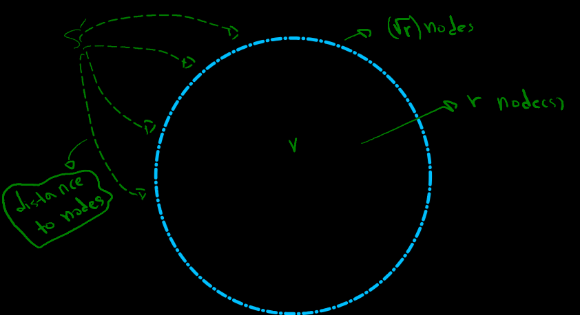
And actually this is possible because we have the information of paths and distances implicitly stored in the distance subgraph, so for each boundary, to go into another boundary we must traverse different pieces from boundary to boundary, so running Dijkstra actually gives us the desired distances.

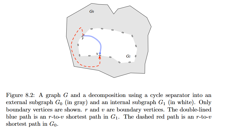
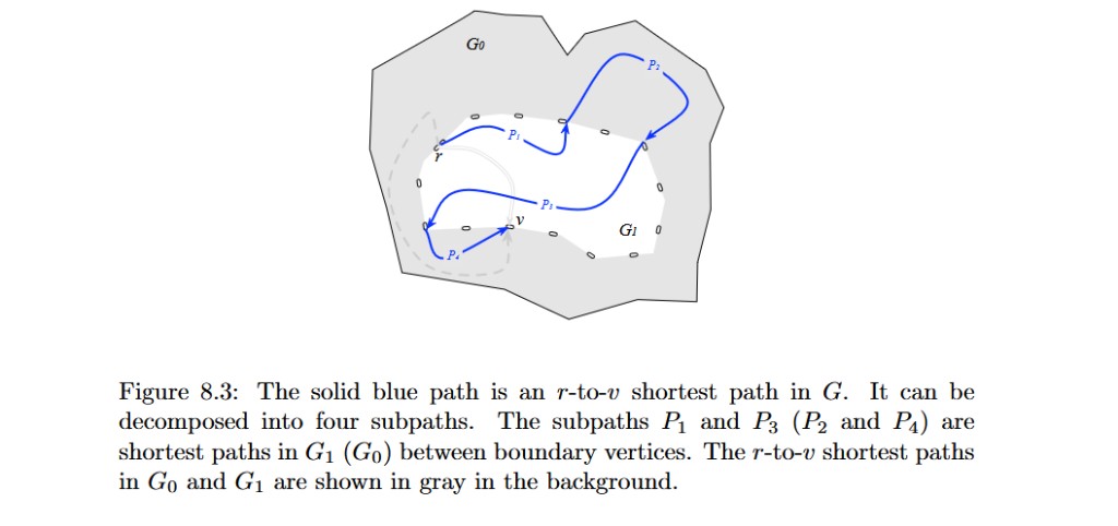
Finally, for each piece \(P\), we attach an artificial source \(s'\) to each boundary vertex \(u\) with an edge of length

where \(d(s,u)\) is the distance from \(s\) to \(u\) computed in the dense distance graph. We then compute a shortest-path tree in \(P\) rooted at \(s'\) using Dijkstra’s algorithm. Since each piece contains \(O(r)\) vertices, this takes

time per piece, or

time overall.

Thus, the overall running time is

In particular, setting

gives

and

Therefore, the total running time is

So as you can see, we incorporated terse sparsified local structures and their information to traverse the graph in a more efficient manner, then when we come sufficiently close, we can consider a piece or region with all of its nodes.

So now here come the ideas of the paper actually. We want to use Dijkstra and Bellman–Ford in case we have negative cases eventually, but we want to do it in a more efficient manner. And one of the more useful techniques of doing so is to bypass the \(O(m)\) complexity of the relaxation phase for each vertex. And to do so, we must use some characteristics of planar graphs. And we will see how we can do it, do kind of bring it down to something like \(O(log(m))\). It’s a rough idea, and so in order to do that we must use the idea of a Monge array, that lets us to do a search like binary search.

A matrix \(M=(M_{ij})\) is totally monotone if for every \(i,i',j,j'\) such that \(i<i'\) and \(j<j'\), if

then

A matrix \(M=(M_{ij})\) is convex Monge (respectively, concave Monge) if for every \(i,i',j,j'\) such that \(i<i'\) and \(j<j'\), we have

(respectively,

\(M_{ij}+M_{i'j'} \le M_{ij'}+M_{i'j}.\))

It is immediate that if \(M\) is convex Monge, then it is totally monotone. It is also easy to see that the matrix obtained by transposing \(M\) is also totally monotone.

Remark. In 1987, Alok Aggarwal, Maria Klawe, Shlomo Moran, Peter Shor, and Robert Wilber described an elegant recursive algorithm that finds the minimum element in every row of an \(n\times n\) Monge array in \(O(n)\) time, now usually called the SMAWK algorithm.

Theorem. For any four indices \(k,k',\ell,\ell'\) such that either \(A_{k\ell}\), \(A_{k\ell'}\), \(A_{k'\ell}\), and \(A_{k'\ell'}\) are all in \(A\)’s upper triangle, or are all in \(A\)’s lower triangle (i.e., either

or

the convex Monge property holds:

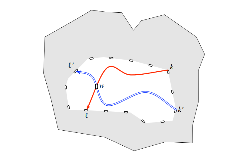
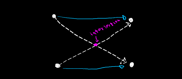
Proof. It is simply a case of using the Jordan curve theorem, finding a middle node or intersection node and uncrossing the nodes to derive the inequality.

The Monge property also implies another important property that we use. That is, for \(y\in B\), if \(u\in A\) is the node that minimizes \(d(u,y)\), then for any \(v\neq u\in A\) and \(x\neq y\in B\),

Given \((A,B,d)\) with the Monge property, the Monge matching problem is to find a parent \(p(v)\in A\) for all \(v\in B\) such that

The set of pairs

forms the minimum Monge matching.

The non-crossing property states that it is enough to look for a function \(p(\cdot)\) that has no “crossing.” Therefore, we can use standard divide-and-conquer techniques to derive an

algorithm for the problem, where

Or constructively we can start from a row to find the min element in the column and use a binary search to add a row, and compute the local minima, which takes the same complexity and is basically the same algorithm.

so ok.

General complete graphs are not Monge. We can preserve the information that the dense distance graph gives us using \(O(\log n)\) Monge arrays, by halving the cycle separator in half and considering only the distances between the two halves and continuing to do this recursively. This way we have at most \(O(\log n)\) levels of Monge matrix, which we can find the possible relaxation candidates simultaneously in \(O(k\log k)\) for which \(k\) is the number of rows and columns in one of the Monge arrays.

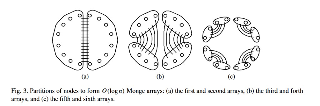
Citing the paper.

We accomplish this by maintaining the edges of each subpiece of \(P\) in \(O(\log n)\) levels of Monge arrays. After the definition of the Monge arrays, we describe how all edges in each Monge array with \(k\) nodes can be relaxed in \(O(k\log k)\) time, where \(k\) is the number of nodes in the data structure.

The first Monge array that we define is formed as follows. Divide the border nodes in some subpiece into two halves, the first (or left) half in the circular order (with an arbitrary starting point) and the second (or right) half. Consider the set of edges in the dense distance graph that go from the left border nodes to the right ones. The edges obey the Monge property, since there is an underlying shortest path tree in which the corresponding paths do not cross.

Using the same left–right partitioning, we can define another Monge array with the direction of edges reversed (i.e., edges in the array go from the right border nodes to the left border nodes).

So, when we want to simulate Dijkstra’s algorithm or Bellman–Ford, we only perform the relaxation operations within these related \(O(\log n)\) data structures.

Therefore, relaxing the edges can be done in

since the total number of nodes in all the data structures is

for each subpiece of \(P\) in the decomposition, and relaxing the edges within a Monge array with \(k\) nodes takes \(O(k\log k)\) time.

In this way, we are handling the information in a very clever manner in order to obtain a better query or time complexity.

Suppose that we have no negative edge; for the other case we have to talk about Bellman–Ford too, which I probably won’t in this chapter or will later update this post.

So how does FR-Dijkstra work?

First of all we must know that things are computed in a clever data structure:

On-line Bipartite Monge Search

It is online in the sense that Dijkstra’s algorithm is online, because in each loop, after relaxation we can find a new node and set it to shortest distance instead of infinity.

An important subroutine in the efficient implementation of Dijkstra’s algorithm running on dense distance graphs is the on-line bipartite Monge search problem.

The algorithm computes shortest paths by combining several instances of the following problem.

Actually the way that we can recursively partition the graph has been improved since the time of the paper publication; they would halve the graph horizontally following the Tarjan–Lipton paper, but we can decompose the planar map cyclically in each step.

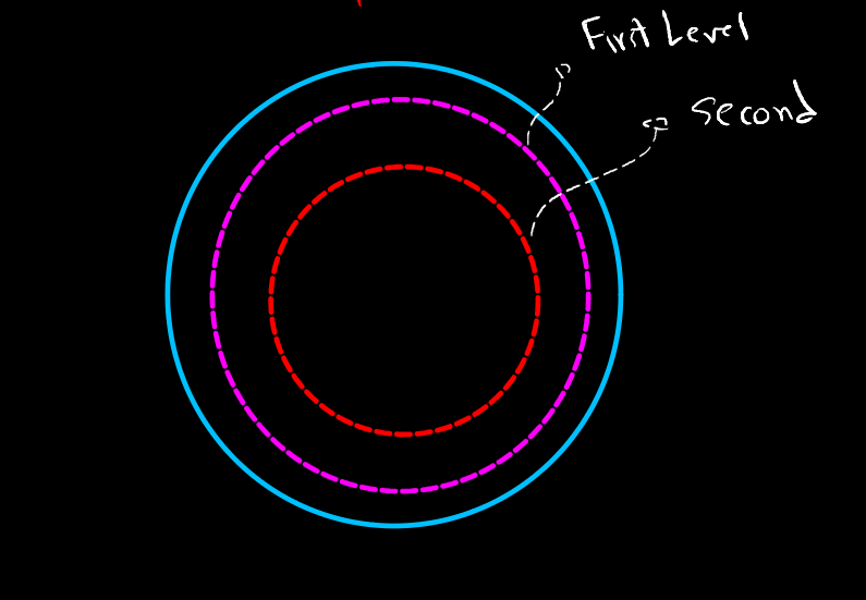
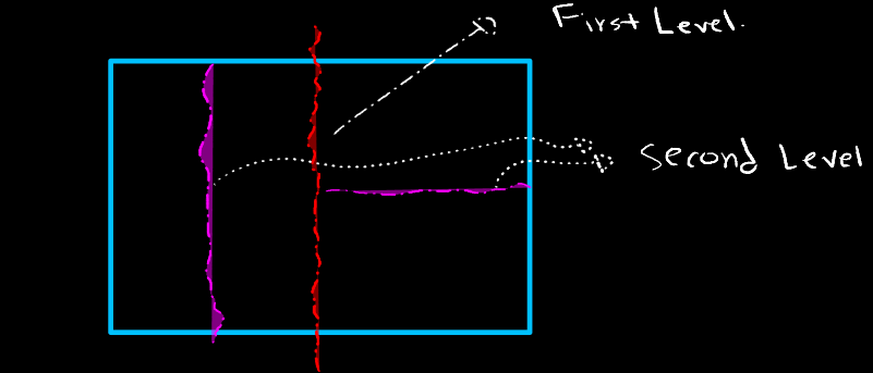
So for each step we can compute the global to local structure of that piece, and we may at most do it \(\log n\) times, so the time complexity would be \(\log n\) times whatever complexity that we get.

And we recursively perform the algorithm that beat Dijkstra recursively to get from one layer to another layer of \(s\)–\(v\) shortest path.

On-line bipartite Monge search. Given \(d(x,y)\), representing a dense distance graph for \(X\times Y\), maintain a parent \(x\in X\) for every \(y\in Y\), while the initialization value \(D(\cdot)\) for each \(x\in X\) is revealed on-line, one node at a time.

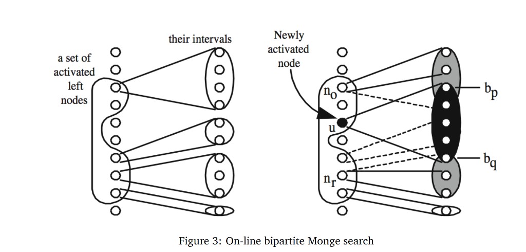
The matching can be computed on-line in overall time

which is the same asymptotic time as the standard divide-and-conquer algorithm.

Maintaining a matching means, in this context, managing:

• a set of active nodes \(A\subseteq X\); and
• a growing set of matched nodes \(M\subseteq Y\), or, more importantly, a shrinking set of yet-unmatched nodes \(Y\setminus M\).

The data structure supports the following three operations, which are used by Dijkstra’s algorithm:

• FindMin(): returns the minimum unmatched node \(y\in Y\setminus M\). This functions as a priority queue for the right-hand side.
• ExtractMin(): adds the current minimum node to \(M\).
• ActivateLeft\((x,\delta)\): reveals the initialization value \(D(x)=\delta\) for some \(x\in X\) and updates the preliminary matches.

Efficient Implementation.

We use a heap and intervals in an ordered set \(Y\). Assume that, for each \(x\in X\), we have precomputed, together with the dense distance graph, a data structure supporting queries of the form

for any \(i^-,i^+\). Note that this data structure is independent of \(D(x)\), and the query can be answered using an LCA data structure in \(O(1)\) time.

Maintain a binary search tree for the active nodes \(x\in A\).

For every active \(x\in A\), maintain an interval

of children \(y\in Y\). Here, \(x\) is the current parent of \(y\), although this parent may change over time.

Maintain a priority queue (heap) containing, for every active \(x\in A\), its shortest edge to an unmatched node \(y\in Y\setminus M\).

• FindMin() returns the minimum element of the heap in \(O(1)\) time.

• ExtractMin() adds the current minimum to \(M\). Suppose the minimum is \(y_j\in Y\setminus M\) with parent \(x\in A\). We need to insert the second-shortest edge from \(x\) into the heap.

  Instead, create two dummy nodes \(x'\) and \(x''\) spanning the intervals

  \[[i^-(x),j) \qquad\text{and}\qquad [j+1,i^+(x)),\]

  respectively. Find the minimum in each of these intervals using the above LCA data structure for \(x\), and insert the resulting edges into the heap. This takes

  \[O(\log |Y|)\]

  time.

  There are at most two new dummy nodes for each extracted node of \(Y\). Hence, there are only

  \[O(|X|+|Y|)\]

  dummy nodes in total.

• ActivateLeft\((x,\delta)\) activates a new node \(x\in X\) with initialization value

  \[D(x)=\delta.\]

  First, compute its interval

  \[[i^-(x),i^+(x)).\]

  If \(x\) is the first active node, the interval contains all of \(Y\). Otherwise, we proceed as follows.

  1. Walk upward through the active nodes with non-empty intervals until reaching the first node \(x'\) such that

     \[d(x',y_{i^-(x')}) < d(x,y_{i^-(x')}).\]

     Then perform a binary search for \(i^-(x)\) in the range

     \[[i^-(x'),i^+(x')).\]

     This takes

     \[O(\log |Y|)\]

     time.

  2. Analogously, walk downward through the active nodes with non-empty intervals until reaching the first node \(x''\) such that

     \[d(x'',y_{i^+(x'')-1}) < d(x,y_{i^+(x'')-1}).\]

     Then perform a binary search for \(i^+(x)\) in the range

     \[[i^-(x''),i^+(x'')).\]

     This also takes

     \[O(\log |Y|)\]

     time.

  Finally, update the other intervals and the heap.

  For nodes in \(A\) between \(x\) and \(x'\) (and between \(x\) and \(x''\)), the corresponding interval becomes empty. These nodes are therefore deactivated, and their corresponding minimum unmatched nodes in \(Y\setminus M\) are removed from the heap.

  Since the sequential search (the “walk up/down”) visits each such node at most once, its total cost is amortized

  \[O(\log |Y|)\]

  per \(x\in X\).

  For \(x'\) and \(x''\), their intervals may shrink to

  \[[i^-(x'),i^-(x)) \qquad\text{and}\qquad [i^+(x)+1,i^+(x'')),\]

  respectively. Either interval may also become empty. The corresponding minimum unmatched node in \(Y\setminus M\) is then updated in the heap, taking

  \[O(\log |Y|)\]

  time.

So really we are keeping a global heap, local heaps for each half of the complete dense graph pieces, making them Monge. And the magic really happens when we are maintaining the parents for the right side of bipartite graphs, which takes \(\log Y\) times amortized. And the algorithm is true because just like the usual Dijkstra it is picking the edges greedily, so only we are using the structure to relax more efficiently.

And the real magic happens when we are handling the parents as I said, Reveal\((j,x)\) is implemented in \(O(\log k)\) amortized time as follows:

• Find the live intervals

  \[I^-=(j^-,i^-_{\min},i^-_{\min}) \qquad\text{and}\qquad I^+=(j^+,i^+_{\min},i^+_{\min})\]

  immediately before and after \((j,\cdot,\cdot)\) in lexicographic order, in \(O(\log k)\) time, by querying the balanced binary search tree.

• While

  \[M[i^-_{\min},j] < M[i^-_{\min},j^-],\]

  replace \(I^-\) with its predecessor in lexicographic order. Then binary search for the smallest index \(i_{\min}\) such that

  \[M[i_{\min},j] < M[i_{\min},j^-].\]

• While

  \[M[i^+_{\min},j] < M[i^+_{\min},j^+],\]

  replace \(I^+\) with its successor in lexicographic order. Then binary search for the smallest index \(i_{\max}\) such that

  \[M[i_{\max},j] < M[i_{\min},j^+].\]

• Delete any live intervals \((j^\pm,\cdot,\cdot)\) that overlap

  \[(j,i_{\min},i_{\max})\]

  from the priority queue.

• Insert the new live intervals

  \[(j,i_{\min},i_{\max}), \qquad (j^-,\cdot,i_{\min}-1), \qquad (j^+,i_{\max}+1,\cdot)\]

  into the priority queue.

To obtain the claimed \(O(\log k)\) amortized time bound, we charge the time required to delete any interval from the priority queue to its earlier insertion. The requirement that we only hide rows when their minimum elements are visible implies that there is exactly one live interval in the revealed column.

FR-Dijkstra\((G,s)\)

for all v in V(G):
    d(v) ← ∞
d(s) ← 0
S ← ∅

Convert each DDG into bipartite DDGs (X_i, Y_i).

for each (X, Y) such that s ∈ Y:
    (X, Y).Insert(s, 0)
    Global.DecreaseKey((X, Y), 0)

while S ≠ V(G):
    (X, Y) ← Global.ExtractMin()
    u ← (X, Y).ExtractMin(Y \ M)

    if u ∉ S:
        for each (X', Y') such that u ∈ X':
            (X', Y').ActivateLeft(u, d(u))
            v ← (X', Y').FindMin(Y' \ M')
            Global.DecreaseKey((X', Y'), d(v))
        S ← S ∪ {u}

    v ← (X, Y).FindMin(Y \ M)
    Global.DecreaseKey((X, Y), d(v))

Sources

• Jittat Fakcharoenphol and Satish Rao, Planar graphs, negative weight edges, shortest paths, and near linear time. Journal of Computer and System Sciences (the 2006 paper this post is about).
• Erik Demaine, MIT 6.889, Lecture 12: Multiple-Source Shortest Paths.
• Philip Klein, Shortest paths in planar graphs with negative lengths.
• Jeff Erickson, computational topology notes: 15 — Shortest paths and 17 — Faster minimum cut.